JIEM, 2015 – 8(4): 1103-1124 – Online ISSN: 2013-0953 – Print ISSN: 2013-8423 http://dx.doi.org/10.3926/jiem.1352
Two-agent Scheduling in Open Shops Subject to Machine
Availability and Eligibility Constraints
Ling-Huey Su, Ming-Chih Hsiao
Chung Yuan Christian University (Taiwan)
[email protected], [email protected]
Received: December 2014
Accepted: July 2015
Abstract:
Purpose:
The aims of this article are to develop a new mathematical formulation and a new
heuristic for the problem of preemptive two-agent scheduling in open shops subject to machine
maintenance and eligibility constraints.
Design/methodology:
Using the ideas of minimum cost flow network and constraint
programming, a heuristic and a network based linear programming are proposed to solve the
problem.
Findings:
Computational experiments show that the heuristic generates a good quality schedule
with a deviation of 0.25% on average from the optimum and the network based linear
programming model can solve problems up to 110 jobs combined with 10 machines without
considering the constraint that each operation can be processed on at most one machine at a
time. In order to satisfy this constraint, a time consuming Constraint Programming is proposed.
F o r
n
= 80 and
m
= 10, the average execution time for the combined models (linear
programming model combined with Constraint programming) exceeds two hours. Therefore,
the heuristic algorithm we developed is very efficient and is in need.
Originality/value:
The main contribution of the article is to split the time horizon into many
time intervals and use the dispatching rule for each time interval in the heuristic algorithm, and
also to combine the minimum cost flow network with the Constraint Programming to solve the
problem optimally.
Keywords:
scheduling, two-agent, open shop, machine availability and eligibility, constraint
programming
1. Introduction
Consider two agents who have to schedule two sets of jobs on an m-machine open shop. Each
job has k operations, k ≤ m, and each operation must be performed on the corresponding
specialized machine. The order in which the operations of each job are performed is irrelevant. Operation preemption is allowed and the machine availability and eligibility constraints are considered. The machine availability arises when machines are subject to breakdowns, maintenance, or perhaps high priority tasks are prescheduled in certain time intervals. The
machine eligibility constraints are imposed when the number of operations of each job i can be
less than m. Each machine can handle at most one operation at a time and each operation can be processed on at most one machine at a time. Two agents are called Agent A and B. Agents A
and B have na(nb) jobs. Let n denote the total number of jobs, i.e., n = na + nb, and each job j of
agent A (B) is denoted by . The processing time of a job j of agent A (B) on machine i is
denoted by . The release time of a job j of agent A (B) is denoted by . Each
machine i is available for processing in the given N(i) intervals, which are , i = 1, ..., m,
k = 1, ..., N(i) and , where and are the start time and end time of the kth availability interval of machine i, respectively. The operations of job j of agent A (B) are
processed on a specified subset of the machines in an arbitrary order. We use
to denote the completion time of Jj for agent A (B) and to
denote the makespan. The objective is to minimize makespan, given that agent B will accept a
schedule of cost up to Q. According to the notation for machine scheduling, the problem is
denoted as , where O indicates open
machines, NCwin means that the machines are not available in certain time intervals, pmtna(b)
signifies job preemption, implies that each job has a release date, denotes the
specific subset of machines to process job j, and denotes agent B will accept a
The multi-agent scheduling problems have received increasing attention recently. Baker and Smith (2003) perhaps the first to consider the problem in which two agents compete on the use of a single machine. They demonstrated that although determining a minimum cost schedule according to any of three criteria: makespan, minimizing maximum lateness, and minimizing total weighted completion time for a single machine, is polynomial, the problem of minimizing a mix of these criteria is NP-hard. Agnetis, Mirchandani, Pacciarelli and Pacifici (2004) studied a two-agent setting for a single machine, two-machine flowshop and two-machine open shop environments. The objective function value of the primary customer is minimized subject to the requirement that the objective function value of the second customer cannot exceed a given number. The objective functions are the maximum of regular functions, the number of late jobs, and the total weighted completion times. The problem in a similar two-agent single machine was further studied by Cheng, Ng and Yuan (2006, 2008), Ng, Cheng and Yuan (2006), Agnetis, Pacciarelli and Pacifici (2007), Agnetis, Pascale and Pacciarelli (2009), Leung, Pinedo and Wan (2010) and Lee, Chung and Huang (2013). When release times are further considered, see (Lee, Chung & Hu, 2012; Yin, Wu, Cheng and Wu, 2012; Yin, Wu, Cheng, Wu & Wu, 2014; Wu, Wu, Chen, Yin & Wu, 2013). The multi-agent problems are extended by considering variations in job processing time such as controllable processing time (Wan, Vakati, Leung & Pinedo, 2010), deteriorating job processing time (Cheng, Wu, Cheng and Wu, 2011; Liu, Yi & Zhou, 2011), and learning effect (Cheng, Cheng, Wu, Hsu and Wu, 2011; Lee & Hsu, 2012; Wu, Huang & Lee, 2011; Yin, Cheng and Wu, 2012). Yu, Zhang, Xu and Yin (2013) considered a two agents problem to minimize an aggregate increasing objection function of two agents’ objective function and a piece-rate maintenance which is implemented once a fixed number of jobs is completed. Mor and Mosheiov (2010) considered minimizing the maximum earliness cost or total weighted earliness cost of one agent, subject to an upper bound on the maximum earliness cost of the other agent. They showed that both minimax and minsum cases are polynomially solvable while the weighted minsum case is NP-hard.
This two-agent problem under consideration arises in TFT-LCD and E-Paper manufacturing wherein units go through a series of diagnostic tests that do not have to be performed in any specified order.
This paper is organized as follows: Section 2 formulates the problem and provides a heuristic. Section 3 is devoted to describing the minimum cost flow network and its corresponding linear programming model. Section 4 illustrates the effectiveness of the heuristic algorithm and computational efficiency of the minimum cost flow network, and finally in Section 5, we provide conclusions.
2. Problem Formulation and the Heuristic Algorithm
First, we rank all , , , , and Q in nondecreasing order and put them into the time
epoch set E. Let el be the lth time epoch in E, i.e., E = {e1, e2, e3, ..., ev}, where el < el+1 and
. Let Tl be the lth time interval between two adjacent time epochs el and el +1,
where l = 1, …, |E|-1. Let m(l) be the set of machines that are available in Tl, i.e., m(l) =
{i|integer k, 1 ≤ k ≤ N(i), such that and }.
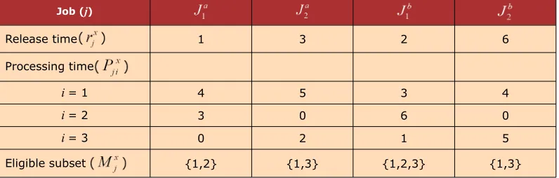
Numerical Example 1. There are two jobs for each agent to be processed on three machines. The job and machine data are listed in Tables 1 and 2 and agent B will accept a schedule of time up toQ = 17.
Job (j)
Release time 1 3 2 6
Processing time
i = 1 4 5 3 4
i = 2 3 0 6 0
i = 3 0 2 1 5
Eligible subset {1,2} {1,3} {1,2,3} {1,3}
Table 1. Job data
Machine (i) i= 1 i= 2 i= 3
Availability interval
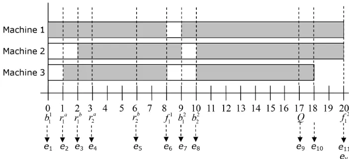
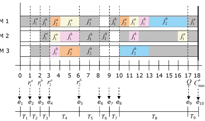
All values of , , and Q are ranked in ascending order. The corresponding time epoch set
E = {e1, e2, e3, ..., e11} = {0, 1, 2, 3, 6, 8, 9, 10, 17, 18, 20}, are shown in Figure 1.
We call operation for job j of agent x, x = a or b, is available on its corresponding machine i
in the time interval Tl if and i Î m(l), where denotes the remaining
unscheduled processing time of operation .
Figure 1. Distinct time epochs in set E
The basic idea of the heuristic is to combine the rule of giving priority to agent B and the rule of the largest remaining processing time first (LRPT) for assigning operations to
machines in each time interval. The rationale of giving priority to agent B is that agent B
only accepts a schedule of cost up to Q. The LRPT rule first selects job j of agent x, ,
which has the maximum remaining processing time and among the available operations of this job, choosing the one which is to be processed on the machine that has maximum
remaining processing time to process. Within each time interval, say Tl, if the completion
time y of the selected operation is less than the time epoch el+1, a new time epoch is set
equal to y and a new time interval is created accordingly, i.e., Tl is split into two time
intervals. That is, if y < el+1, set el+1 = y, el+2 = el+1, el+3 = el+2, …, ev+1 = ev. The steps of the
heuristic algorithm are as follows.
Step 1. Rank , , and Q in ascending order, and put into the time epoch E. Let
Step 2. If no operation is available to the time interval Tl, set l = l + 1 and return to Step 2. If
any operation of agent b available to the time interval Tl([el,el+1]), set x = b, otherwise set x = a.
Use the LRPT rule to find the operation of agent x to be processed on the machine, say
machine i, in the time interval Tl. S e t , , ,
and . If for j = 1, 2, …, nx, x = a, b; the heuristic algorithm
is terminated and . If , go to Step 3 to create a new interval; otherwise
i f , then go to Step 2 until the available operations of agent x in this time interval Tl
have been considered. If x = b, then continue the assignment of operations in the same manner for x = a in time interval Tl. Set l = l + 1 and go to Step 2.
Step 3. Let el+1 = , el+2 = el+1, el+3 = el+2, ..., ev+1 = ev, E = {el+1, el+2, ..., ev+1, }, and go to Step 2.
We demonstrate the heuristic algorithm using the data of Numerical Example 1.
Numerical Example 2. The values of the total remaining unscheduled processing time of job j
for both agents are = 7, =7, =10 and = 9.
Iteration 1
Step 1. The corresponding time epoch set E = {e1, e2, e3, ..., e11} = {0, 1, 2, 3, 6, 8, 9, 10, 17, 18, 20} is
shown in Figure 1. Set l = 1.
Step 2. Since there is no available operation in [e1, e2], set l = 2. In [e2, e3], no operation for
agent B is available and thus is selected to be processed on m1 due to the maximum value
of and the maximum machine load of m1. Since y = 1, update the values of , and
a s 3, 6 and 2, respectively. Since there is no more available operation in the time interval
[e2, e3], we set l = 3. Using the same manner, the time interval [e3, e4], [e4, e5], [e5, e6], [e6, e7] and
[e7,e8] are scheduled. In the time interval [e8, e9], the available jobs for agent B are and
is selected to be processed on m3. Since y = 3, update the values of , and as 0, 3
and 13, respectively. Since E, therefore return to Step 3.
Step 3. Let e9 equal to = 13 and re-index time epochs in E. That is [e10, e9], [e11, e10], [e12, e11],
Iteration 2
Step 2. In [e8, e9], is selected to be processed on m2, however, is not in set E, therefore go
to Step 3.
Step 3. Let e9 equal to = 11, E = {11, 13, 17, 18, 20}, and return to Step 2.
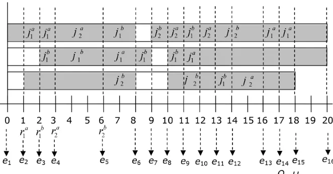
Proceed in the same manner, the heuristic solution with Cmax = 18 is obtained and shown in
Figure 2.
3. The Exact Algorithm
In this section, we develop a linear programming model based on minimum cost flow network to test the effectiveness of the heuristic. For the problem of the parallel-machine scheduling problem, P, NCwin|pmtn, rj, Mj|Cmax, Liao and Sheen (2008) solved the problem by first
formulating a base problem with respect to a given Cmax as a maximum flow problem. They
then proposed a binary search algorithm to test the feasibility of the problem and to determine the optimal makespan by solving a series of maximum network flow problems. Su, Cheng and Chou (2013) revised their maximum flow model to the minimum cost flow model for the same problem with makespan and maximum lateness criteria. We further extend their network for the two-agent open shop problem to test the effectiveness of our heuristic algorithm.
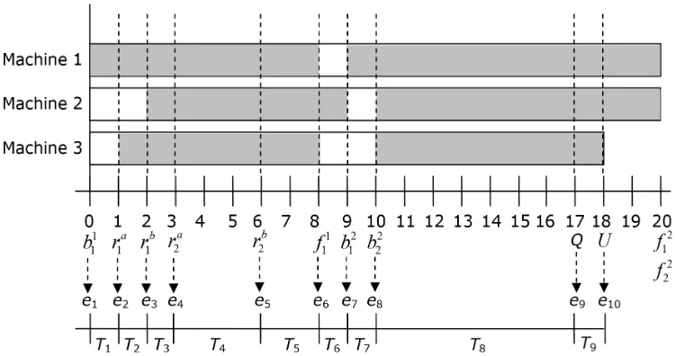
First, we set U, the solution of the heuristic algorithm, as an upper bound on the makespan.
Next, we rank all , , , , Q and U in increasing order and put them into the time epoch
set E as previously described. E = {e1, e2, e3, ..., ev}, where el < el+1 and ev = U. The time epochs
in the time interval from U to are redundant and can be discarded. Using the data of
the Numerical Example 1, the diagram of the time epoch set E and the time intervals Tl is
shown in Figure 3.
Figure 3. Distinct time epochs in set E for Numerical Example 1
Upon obtaining E, Tl and m(l), we formulate the problem with U as a minimum cost flow
The network consists of a set of nodes and a set of arcs connecting certain pairs of the nodes.
The node set in G(U) includes a source node s, a sink node t, and the following three node sets.
(i) Job nodes, , j = 1, 2, …, nx, x = a, b.
(ii) Combination nodes consisting of job ,j = 1, 2, …, nx, x = a, b and time
interval Tl, where Tl satisfies el+1 ≤ U and ≤ el for agent A and el+1 ≤ Q and ≤ el
for agent B.
(iii) Combination nodes (i, Tl) consisting of machine i and time interval Tl, where Tl satisfies
el+1 ≤ U and iÎm(l).
The arc set consists of directed arcs that are generated as follows.
(i) An arc with capacity for j = 1, 2, …, nx, x = a, b.
(ii) An arc from node to node with capacity (el+1 – el).
(iii) An arc from node to (i, Tl) with capacity (el+1 – el) if and only if
iÎ m(l).
(iv) An arc ((i, Tl), t) from node (i, Tl) to the sink t with capacity (el+1 – el), i = 1, 2, …, m.
(v) Finally, there is an arc (s,t) from node s to node twith capacity ∞.
The source node s consists of n + 1 emanating arcs. Let f(x, y) denote the flow in the arc from
nodex to node y, i.e. nodex and node y are a pair of nodes connecting this arc. A positive f(s,t)
indicates that an amount of flow equal to f(s, t) cannot be assigned to the machines under the
upper bound U, i.e. there exists no feasible schedule in which the completion time of each job is no greater than U. This happens if U is a trial value which is incorrectly set or the heuristic algorithm is incorrectly calculated. Denote the latest arrival times of agent A and B and the
The corresponding directed tripartite network G(U) using the data of Numerical Example 1 is
shown in Figure 4. Figure 4. The optimal solution for Numerical Example 1
Using the convention that summations are taken only over existing arcs, we formulate
O, NCwin|pmtna, , : pmtnb, , |Cmax : ≤ Q as a linear programming problem, called LP,
Minimize
(1)
Subject to
(2)
(3)
, for node
, for node (4)
, for node (5)
(6)
(7)
(8)
(9)
(10)
In the first term of the objective Function (1), we assign an arbitrarily large cost M to the
arc f(s, t) to ensure that the maximum feasible flow goes through all the other arcs , j =
1, 2, …, nx, x = a, b. The summations in the latter terms ensure the assignment of jobs to time
intervals as early as possible, where ε denotes an arbitrarily small number. As an illustration, refer to Numerical Example 1 and Figure 4. The latter term of the objective Function (1) for
Numerical Example 1 i s , in which the cost is given to the time
intervals from T6 to T9. The time epochs from the last arrival time to the upper bound of is
e5 to e10, associated with time intervals from T5 to T9. Since e5 is the last arrival time and some
operations will definitely be scheduled in T5, therefore the cost is imposed to the time interval
from T6 to T9. We give cost ε, 2ε, 3ε and 4ε to the time interval T6, T7, T8 and T9, respectively, to
ensure the assignment of operations to these time intervals as early as possible. Constraints (2) guarantee that the total processing times of all operations of both agents should be assigned to machines in different time intervals. Constraints (3)-(6) are the mass balance constraints. Constraints (7)-(11) represent the capacity constraints.
I f f(s, t) is zero, the n the o ptimal makespan is , where
such that f((i, Tk), t) > 0 for i = 1, 2, …, m}. For illustration, as Figure
4 shows, the basic variables of the optimal solution are depicted by the thick lines.
such that f((i, Tk), t) > 0 for i = 1, 2, 3} = 9, and =
e9 + 1 = 17 + 1= 18.
The linear programming model with 1 + n × v + m × (n + 1) × (v – 1) variables, including n for arcs , n ×(v – 1) for arcs , m × (v – 1) for arcs ((i, Tl), t), and one for arc (s, t), and
3 + 2 × v (n + m) + m ×(n × v – 2) constraints for all functional constraints from (2) to (11).
Figure 5. Gantt diagram of the optimal solution for Example 1
As Figure 5 shows, operation is processed on machines 1 and 2, operation is processed
on machines 1 and 3, and operation is processed on machine 2 and 3 in time interval T4. In
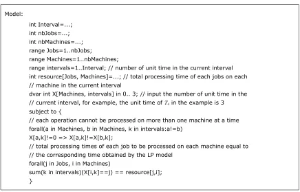
order to satisfy the constraint that each operation can be processed on at most one machine at a time, we use Constraint Programming (Brailsford, Potts & Smith, 1999; Van Hentenryck, 2002) to solve this problem. Constraint Programming generates a schedule that satisfies the above constraint in each time interval. The model in Figure 6 is coded for this purpose.
Model:
int Interval=...; int nbJobs=...; int nbMachines=...; range Jobs=1..nbJobs;
range Machines=1..nbMachines;
range intervals=1..Interval; // number of unit time in the current interval int resource[Jobs, Machines]=...; // total processing time of each jobs on each // machine in the current interval
dvar int X[Machines, intervals] in 0.. 3; // input the number of unit time in the // current interval, for example, the unit time of T4 in the example is 3 subject to {
// each operation cannot be processed on more than one machine at a time forall(a in Machines, b in Machines, k in intervals:a!=b)
X[a,k]!=0 => X[a,k]!=X[b,k];
// total processing times of each job to be processed on each machine equal to // the corresponding time obtained by the LP model
forall(j in Jobs, i in Machines)
We coded the algorithm in ILOG OPL Studio 6.1 and ran it on a PC with AMD 2.91GHz. The
Gantt diagram of the optimal solution is shown in Figure 7, where the time interval T8 is
implemented using the same model.
Figure 7. Gantt diagram of the optimal solution for Example 1
4. Computational Results
The objective of the computational experiments described in this section is to evaluate both the performances of the heuristic and the exact algorithms. All experimental tests were run on a personal computer with AMD 2.91GHz CPU. The heuristic algorithm was coded in Visual Basic, and the linear programming model and the constraint programming model were solved by LINGO11.0 and ILOG OPL 6.1, respectively. The experiment involves the instances with the number of jobs n = 40, 60, 80, 100 and 110 in which three pairs of na and nb are set as
{(na = 20, nb = 20), (na = 25, nb = 15), and (na = 15, nb = 25)},
{(na = 30, nb = 30), (na = 35, nb = 25), and (na = 25, nb = 35)},
{(na = 40, nb = 40), (na = 45, nb = 35), and (na = 35, nb = 45)},
{(na = 50, nb = 50), (na = 60, nb = 40), and (na = 40, nb = 60)}, and
The processing time of are randomly generated from an uniform distribution U[0, 10]. The
job arrival time refers to Chu (1992) and are generated from U[0, ], where
is the mean processing time on each machine. The number of
machine m is set as m = 6, 8 and 10. To generate the upper bound of makespan for agent b, we
refer to Bank and Werner (2001) with
,
where and β Î {1.2, 1.5, 2, 2.5}. The rate of machine availability θ is
set as 0.7, 0.9 and 1.0. Five instances are generated for each combination of n, m, , , θ, Q, yielding 900 instances. In comparing heuristic performance, the following formula is used to determine the deviation of the heuristic solution over the optimal solution.
Deviation (%) = [(heuristic-optimum)/optimum] ×100%.
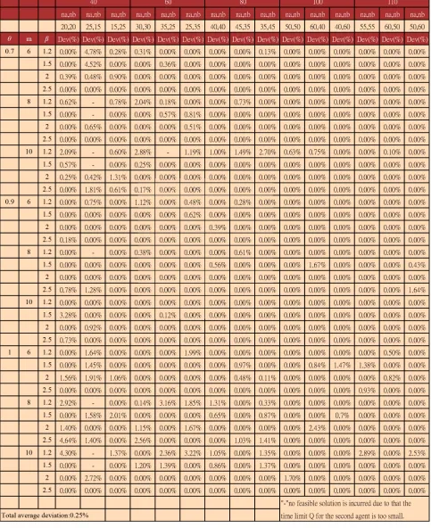
Table 3 shows the solution quality of the heuristic. The influences of m, n, na/nb and θ on the
Table 3 illustrates that the deviation of the heuristic from the optimal solution appears in descending trend as the value of m increases. The reason is that the heuristic selects the maximum total remaining processing time of each job, instead of that of each machine, to be
processed on the corresponding machine. For the rate of machine availability θ, the value of
1 showing that all machines are available at any times. Since none of , i = 1, ..., m, k = 1, ..., N(i) incurred, the number of time intervals decreases and the span of time interval increases, therefore more jobs are competing to be scheduled in each time interval and hence the error increases. As to the number of jobs, the higher value that n is, the better the performance of the heuristic. One reason is that the higher value for n implies more time
epochs incurred and a smaller time span for each Tl making the heuristic easier to assigning
the operations correctly. Another reason is that the denominator increases, whereas the deviation of the heuristic solution from the optimal solution may not increase in proportion to the denominator. There is no significant difference in the performance of the heuristic on the value of na/nb, but na/nb = 0.5 gives the best performance. When na/nb increases, the deviation
increases due to the fact that the heuristic gives priority to agent B and thus more operations
of agent A should compete to schedule in each time interval.
Based on this analysis, we found that decreasing machine number m and the value of na/nb
reduced the deviation of the heuristic, while decreasing job number n increased the deviation of the heuristic. The heuristic generates a good quality schedule with a deviation from the
optimum of 0.25% on average.
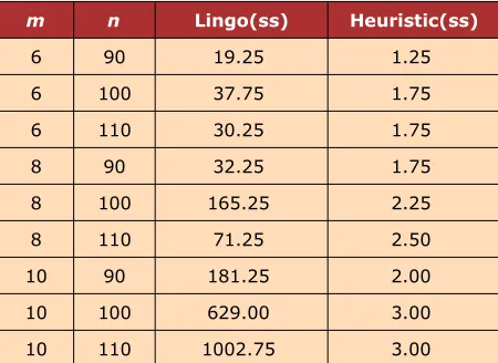
As to the execution time of the heuristic, Table 4 shows the average execution time of the network based linear programming and the heuristic. The average execution time of the heuristic is small compared to that of the linear programming.
m n Lingo(ss) Heuristic(ss)
6 90 19.25 1.25
6 100 37.75 1.75
6 110 30.25 1.75
8 90 32.25 1.75
8 100 165.25 2.25
8 110 71.25 2.50
10 90 181.25 2.00
10 100 629.00 3.00
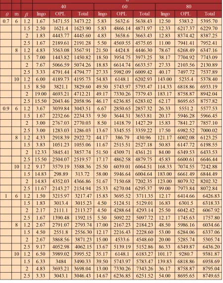
In Table 5, the average execution times in seconds for Linear Programming model, Constraint Programming model, and Combined model (Linear programming and Constraint Programming)
are shown in columns lingo, OPL, and Total, respectively. For n = 80 and m = 10, the average
execution time for the combined model exceeds two hours. Therefore, an efficient heuristic algorithm is in great need.
5. Conclusion
In this paper, we have analyzed the preemptive open-shop with machine availability and eligibility constraints for two-agent scheduling problem. The objective is to minimize makespan, given that one agent will accept a schedule of time up to Q. This problem arises in TFT-LCD and E-Paper manufacturing wherein units go through a series of diagnostic tests that do not have to be performed in any specified order. We proposed an effective heuristic to find a nearly optimal solution and a linear programming model based on minimum cost flow network to optimally solve the problem. Computational experiments show that the heuristic generates a good quality schedule with a deviation of 0.25% on average from the optimum.
References
Agnetis, A., Mirchandani, P.B., Pacciarelli, D., & Pacifici, A. (2004). Scheduling problems with
two competing agents. Operations Research, 52(2), 229-242.
http://dx.doi.org/10.1287/opre.1030.0092
Agnetis, A., Pacciarelli, D., & Pacifici, A. (2007). Multi-agent single machine scheduling. Annals
of Operations Research, 150(1), 3-15. http://dx.doi.org/10.1007/s10479-006-0164-y
Agnetis, A., Pascale, de G., & Pacciarelli, D. (2009). A Lagrangian approach to single-machine
scheduling problems with two competing agents. Journal of Scheduling, 12(4), 401-415.
http://dx.doi.org/10.1007/s10951-008-0098-0
Brailsford, S.C., Potts, C.N., & Smith, B.M. (1999). Constraint satisfaction problems:
Algorithms and applications. European Journal of Operational Research, 119(3), 557-581.
http://dx.doi.org/10.1016/S0377-2217(98)00364-6
Bank, J., & Werner, F. (2001). Heuristic Algorithms for Unrelated Parallel Machine Scheduling with a Common Due Date, Release Dates, and Linear Earliness and Tardiness Penalties. Mathematical and Computer Modelling, 33(4-5), 363-383. http://dx.doi.org/10.1016/S0895-7177(00)00250-8
Breit, J., Schmidt, G., & Strusevich, V.A. (2001). Two-machine open shop scheduling with an
availability constraint. Operations Research Letters, 29(2), 65-77.
http://dx.doi.org/10.1016/S0167-6377(01)00079-7
Baker, K.R., & Smith, J.C. (2003). A multiple-criterion model for machine scheduling. Journal
of Scheduling, 6(1), 7-16. http://dx.doi.org/10.1023/A:1022231419049
Cheng, T.C.E., Ng, C.T., & Yuan, J.J. (2006). Multi-agent scheduling on a single machine to
minimize total weighted number of tardy jobs. Theoretical Computer Science, 362(1-3),
273-281. http://dx.doi.org/10.1016/j.tcs.2006.07.011
Cheng, T.C.E., Ng, C.T., & Yuan, J.J. (2008). Multi-agent scheduling on a single machine with
max-form criteria. European Journal of Operational Research, 188(2), 603-609.
http://dx.doi.org/10.1016/j.ejor.2007.04.040
Cheng, T.C.E., Cheng, S.R., Wu, W.H., Hsu, P.H., & Wu, C.C. (2011). A two-agent single-machine scheduling problem with truncated sum-of-processing-times-based learning
considerations. Computers & Industrial Engineering, 60(4), 534-541.
http://dx.doi.org/10.1016/j.cie.2010.12.008
Cheng, T.C.E., Wu, W.H., Cheng, S.R., & Wu, C.C. (2011). Two-agent scheduling with
position-based deteriorating jobs and learning effects. Applied Mathematics and Computation,
217(21), 8804-8824. http://dx.doi.org/10.1016/j.amc.2011.04.005
Gonzalez, T., & Sahni, S. (1976). Open shop scheduling to minimize finish time. Annals of Operations Research, 23(4), 665-679. http://dx.doi.org/10.1145/321978.321985
Liao, L.W., & Sheen, G.J. (2008). Parallel machine scheduling with machine availability and
eligibility constraints. European Journal of Operational Research, 184(2), 458-467.
http://dx.doi.org/10.1016/j.ejor.2006.11.027
Leung, J.Y.T., Pinedo, M., & Wan, G.H. (2010). Competitive Two-Agent Scheduling and Its
Applications. Operations Research, 58(2), 458-469. http://dx.doi.org/10.1287/opre.1090.0744
Lee, D.C., & Hsu, P.H. (2012). Solving a two-agent single-machine scheduling problem
considering learning effect. Computers & Operations Research, 39, 1644-1651.
http://dx.doi.org/10.1016/j.cor.2011.09.018
Lee, W.C., Chung, Y.H., & Hu, M.C. (2012). Genetic algorithms for a two-agent single-machine
problem with release time. Applied Soft Computing, 12, 3580-3589.
http://dx.doi.org/10.1016/j.asoc.2012.06.015
Lee, W.C., Chung, Y.H., & Huang, Z.R. (2013). A single-machine bi-criterion scheduling
problem with two agents. Applied Mathematics and Computation, 219, 10831-10841.
http://dx.doi.org/10.1016/j.amc.2013.05.025
Liu, P., Yi, N., & Zhou, X. (2011). Two-agent single-machine scheduling problems under
increasing linear deterioration. Applied Mathematical Modelling, 35, 2290-2296.
Mor, B., & Mosheiov, G. (2010). Scheduling problems with two competing agents to minimize
minmax and minsum earliness measures. European Journal of Operational Research, 206(3),
540-546. http://dx.doi.org/10.1016/j.ejor.2010.03.003
Ng, C.T., Cheng, T.C.E., & Yuan, J.J. (2006). A note on the complexity of the problem of
two-agent scheduling on a single machine. Journal of Combinatorial Optimization, 12(4),
386-393. http://dx.doi.org/10.1007/s10878-006-9001-0
Sedeno-Noda, A., Alcaide, D., & Gonzalez-Martin, C. (2006). Network flow approaches to
pre-emptive open-shop scheduling problems with time-windows. European Journal of
Operational Research, 174(3), 1501-1518. http://dx.doi.org/10.1016/j.ejor.2005.01.062
Sedeno-Noda, A., Pablo, de D.A.L., & Gonzalez-Martin, C. (2009). A network flow-based method to solve performance cost and makespan open-shop scheduling problems with
time-windows. European Journal of Operational Research, 196(1), 140-154.
http://dx.doi.org/10.1016/j.ejor.2008.02.031
Su, L.H., Cheng, T.C.E., & Chou, F.D. (2013). A minimum-cost network flow approach to
preemptive parallel-machine scheduling. Computers and Industrial Engineering, 64, 453-458.
http://dx.doi.org/10.1016/j.cie.2012.04.020
Van Hentenryck, P. (2002). Constraint and integer programming in OPL. Informs Journal on
Computing, 14(4), 345-372. http://dx.doi.org/10.1287/ijoc.14.4.345.2826
Wan, G.H., Vakati, S.R., Leung, J.Y.T., & Pinedo, M. (2010). Scheduling two agents with
controllable processing times. European Journal of Operational Research, 205(3), 528-539.
http://dx.doi.org/10.1016/j.ejor.2010.01.005
Wu, C.C., Huang, S.K., & Lee, W.C. (2011). Two-agent scheduling with learning consideration. Computers & Industrial Engineering, 61, 1324-1335. http://dx.doi.org/10.1016/j.cie.2011.08.007
Wu, C.C., Wu, W.H., Chen, J.C., Yin, Y., & Wu, W.H. (2013). A study of the single-machine
two-agent scheduling with release times. Applied Soft Computing, 13, 998-1006.
http://dx.doi.org/10.1016/j.asoc.2012.10.003
Yin, Y., Cheng, S.R., & Wu, C.C. (2012). Scheduling problems with two agents and a linear
non-increasing deterioration to minimize earliness penalties. Information Sciences, 189,
282-292. http://dx.doi.org/10.1016/j.ins.2011.11.035
Yin, Y., Wu, W.H., Cheng, S.R., & Wu, C.C. (2012). An investigation on a two-agent
single-machine scheduling problem with unequal release dates. Computers & Operations
Yin, Y., Wu, W.H., Cheng, T.C.E., Wu, C.C., & Wu, W.H. (2014). A honey-bees optimization
algorithm for a two-agent single-machine scheduling problem with ready times. Applied
Mathematical Modelling. http://dx.doi.org/10.1016/j.apm.2014.10.044
Yu, X., Zhang, Y., Xu, D., & Yin, Y. (2013). Single machine scheduling problem with two
synergetic agents and piece-rate maintenance. Applied Mathematical Modelling, 37,
1390-1399. http://dx.doi.org/10.1016/j.apm.2012.04.009
Journal of Industrial Engineering and Management, 2015 (www.jiem.org)
Article's contents are provided on a Attribution-Non Commercial 3.0 Creative commons license. Readers are allowed to copy, distribute and communicate article's contents, provided the author's and Journal of Industrial Engineering and Management's names are included.