Parametric, Vector, and Polar Functions

530

Chapter

I

n 1935, air traffic control was conducted with a

system of teletype machines, wall-sized

black-boards, large table maps, and movable markers

representing airplanes. Today’s radar data

pro-cessing includes an automatic display of aircraft

identification, speed, altitude, and velocity vectors.

A DC-10 plane flying due west at 600 mph

en-ters a region with a steady air current coming from

the southwest at 100 mph. How should the pilot

adjust the airplane’s course and speed to maintain

its original velocity vector? This type of problem is

covered in Section 10.2.

Parametric,

Vector, and Polar

Functions

Section 10.1 Parametric Functions 531

Chapter 10 Overview

The material in this book is generally described as the calculus of a single variable, since it

deals with functions of one independent variable (usually

x

or

t

). In this chapter you will apply

your understanding of single-variable calculus in three kinds of two-variable contexts, enabling

you to analyze some new kinds of curves (parametrically defined and polar) and to analyze

motion in the plane that does not proceed along a straight line. Interestingly enough, this will

not require the tools of multi-variable calculus, which you will probably learn in your next

cal-culus course. We will simply use single-variable calcal-culus in some new and interesting ways.

Parametric Functions

Parametric Curves in the Plane

We reviewed parametrically defined functions in Section 1.4. Instead of defining the

points (

x

,

y

) on a planar curve by relating

y

directly to

x

, we can define both coordinates as

functions of a parameter

t

. The resulting set of points may or may not define

y

as a

func-tion of

x

(that is, the parametric curve might fail the vertical line test).

10.1

What you’ll learn about

• Parametric Curves in the Plane

• Slope and Concavity

• Arc Length

• Cycloids

. . . and why

Parametric equations enable us

to define some interesting and

important curves that would be

difficult or impossible to define in

the form y

f

(x).

EXAMPLE 1

Reviewing Some Parametric Curves

Sketch the parametric curves and identify those which define

y

as a function of

x

. In

each case, eliminate the parameter to find an equation that relates

x

and

y

directly.

(a)

x

cos

t

and

y

sin

t

for

t

in the interval [0, 2

)

(b)

x

3 cos

t

and

y

2 sin

t

for

t

in the interval [0, 4

]

(c)

x

t

and

y

t

2 for

t

in the interval [0, 4]

SOLUTION

(a)

This is probably the best-known parametrization of all. The curve is the unit circle

(Figure 10.1a), and it does not define

y

as a function of

x

. To eliminate the parameter, we

use the identity

cos

t

2

_sin

_t

2

_{1 to write}

_x

2

_y

2

_1.

(b)

This parametrization stretches the unit circle by a factor of 3 horizontally and by a factor

of 2 vertically. The result is an ellipse (Figure 10.1b), which is traced twice as

t

covers the

in-terval [0, 4

]. (In fact, the point (3, 0) is visited three times.) It does not define

y

as a

function of

x

. We use the same identity as in part (a) to write

3

x

2

2

y

2

1.

(c)

This parametrization produces a segment of a parabola (Figure 10.1c). It does define

y

as a function of

x

. Since

t

x

2

_{, we write}

_y

_x

2

_2.

_{Now try Exercise 1.}

Figure 10.1 A collection of parametric curves (Example 1). Each point (x,y) is determined by parametric functions of t, but only the parametrization in graph (c) determines yas a function of x.

3

–3 –2

(a) y

x

(b)

4 1

– 4 –1

–3 3

1 x

y

2 1

–1 –2

3

–3

(c) y

x

Slope and Concavity

We can analyze the slope and concavity of parametric curves just as we can with

explicitly-defined curves. The slope of the curve is still

dy

dx

, and the concavity still depends on

d

2

_y

_dx

2

_{, so all that is needed is a way of differentiating with respect to}

_x

_{when everything}

is given in terms of

t

. The required parametric differentiation formulas are straightforward

applications of the Chain Rule.

EXAMPLE 2

Analyzing a Parametric Curve

Consider the curve defined parametrically by

x

t

2

_{5 and}

_y

_{2 sin}

_t

_{for 0}

_t

_.

(a)

Sketch a graph of the curve in the viewing window [

7, 7] by [

4, 4]. Indicate the

direction in which it is traced.

(b)

Find the highest point on the curve. Justify your answer.

(c)

Find all points of inflection on the curve. Justify your answer.

SOLUTION

(a)

The curve is shown in Figure 10.2.

(b)

We seek to maximize

y

as a function of

t

, so we compute

dy

dt

2 cos

t

. Since

dy

dt

is positive for 0

t

2 and negative for

2

t

, the maximum occurs when

t

2. Substituting this

t

value into the parametrization, we find the highest point to be

approximately (

2.533, 2).

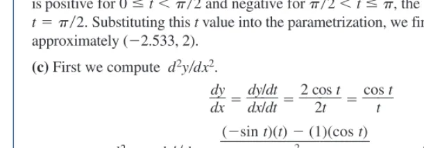
(c)

First we compute

d

2

_y

_dx

2

_.

_d

d

y

_x

d

_d

y

_x

_/

/

d

_d

_t

t

2 c

₂

o

_t

s

t

co

_t

s

t

d

dx

2

_y

2

d

d

y

x

d

d

t

t

t

sin

t

2

t

3

cos

t

2

t

A graph of

y

t

sin

t

2

t

3

cos

t

on the interval [0,

] (Figure 10.3)

shows a sign change at

t

2.798386... . Substituting this

t

value into the

parametriza-tion, we find the point of inflection to be approximately (2.831, 0.673).

Now try Exercise 19.

(

sin

t

)(

t

)

(1)(cos

t

)

t

2

[0, p] by [– 0.1, 0.1]

Figure 10.3 The graph of d2_y

_dx2 _{for the}

parametric curve in Example 2 shows a sign change at t2.798386 ... , indicating a point of inflection on the curve. (Example 2)

Parametric Differentiation Formulas

If

x

and

y

are both differentiable functions of

t

and if

dx

dt

0, then

d

d

y

x

d

d

x

y

d

d

t

t

.

If

y

dy

dx

is also a differentiable function of

t

, then

d

dx

2

_y

2

d

d

x

(

y

)

d

d

y

x

d

d

[image:3.684.212.518.464.571.2]

t

t

.

Figure 10.2 The parametric curve defined in Example 2.

6 1

1

– 6 0

–3 3 y

x

Arc Length

Section 10.1 Parametric Functions 533

Here is a third formula based on the same approximation.

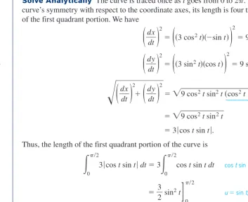
EXAMPLE 3

Measuring a Parametric Curve

Find the length of the astroid (Figure 10.5)

x

cos

3

_t

_,

_y

_sin

3

_t

_,

₀

_t

₂

_.

SOLUTION

Solve Analytically

The curve is traced once as

t

goes from 0 to 2

. Because of the

curve’s symmetry with respect to the coordinate axes, its length is four times the length

of the first quadrant portion. We have

(

d

_d

x

_t

)

2

(

3 cos

2

_t

_sin

_t

)

2

9 cos

4

_t

_sin

2

_t

(

d

_d

y

_t

)

2

(

3 sin

2

_t

_cos

_t

)

2

9 sin

4

_t

_cos

2

_t

(

d

_d

x

_t

)

2

(

d

_d

y

_t

)

2

9

c

o

s

2

_t

_s

_in

2

_t

_c

_o

_s

2

_t

_s

_in

2

_t

1

9

c

o

s

2

_t

_s

_in

2

_t

3

cos

t

sin

t

.

Thus, the length of the first quadrant portion of the curve is

p2

0

3

cos

t

sin

t

dt

3

p2 0

cos

t

sin

t dt

costsint0, 0t/2

3

2

sin

2

_t

]

p2 0

usint, ducost dt

3

2

.

The length of the astroid is 4

3

2

6.

Support Numerically

NINT

3

cos

t

sin

t

,

t

, 0, 2

6.

Now try Exercise 29. x

y

yf (x)

0 (a, c)

(b, d)

c d

a

√⎯⎯⎯⎯⎯⎯⎯⎯⎯⎯⎯(x )_k2 _{(y )}

k2

b x_k x_{k – 1}

x_k y_k Q

[image:4.684.70.575.44.660.2]

P

Figure 10.4 The graph of f, approxi-mated by line segments.

Arc Length of a Parametrized Curve

Let

L

be the length of a parametric curve that is traversed exactly once as

t

increases

from

t

₁

to

t

₂

.

If

dx

dt

and

dy

dt

are continuous functions of

t

, then

L

t₂

t₁

(

d

d

x

t

)

2

(

d

d

y

t

)

2

dt.

Cycloids

Suppose that a wheel of radius

a

rolls along a horizontal line without slipping (see

Figure 10.6

. The path traced by a point

P

on the wheel’s edge is a

cycloid

, where

P

is

originally at the origin.

[image:4.684.217.570.312.600.2]

x = cos3 _{t, y = sin}3 _{t, 0 ≤ t ≤ 2p}

Figure 10.5 The astroid in Example 3.

y

O

P(x, y)

at

a t

C(at, a)

x

Figure 10.6 The position of P(x,y) on the edge of the wheel when the wheel has turned t radians. (Example 4)

EXAMPLE 4

Finding Parametric Equations for a Cycloid

Find parametric equations for the path of the point

P

in Figure 10.6.

SOLUTION

We suppose that the wheel rolls to the right,

P

being at the origin when the turn angle

t

equals 0. Figure 10.6 shows the wheel after it has turned

t

radians. The base of the wheel is

at distance

at

from the origin. The wheel’s center is at (

at

,

a

, and the coordinates of

P

are

x

at

a

cos

,

y

a

a

sin

.

To express

in terms of

t

, we observe that

t

3

2

2

k

for some integer

k

, so

3

₂

t

2

k

.

Thus,

cos

cos

(

3

2

t

2

k

)

sin

t

,

sin

sin

(

3

2

t

2

k

)

cos

t

.

Therefore,

x

at

a

sin

t

a

t

sin

t

,

y

a

a

cos

t

a

1

cos

t

.

Now try Exercise 41.

Investigating Cycloids

Consider the cycloids with parametric equations

x

a

t

sin

t

,

y

a

1

cos

t

,

a

0.

1.

Graph the equations for

a

1, 2, and 3.

2.

Find the

x

-intercepts.

3.

Show that

y

0 for all

t

.

4.

Explain why the arches of a cycloid are congruent.

5.

What is the maximum value of

y

? Where is it attained?

6.

Describe the graph of a cycloid.

EXPLORATION 1

EXAMPLE 5

Finding Length

Find the length of one arch of the cycloid

x

a

t

sin

t

,

y

a

1

cos

t

,

a

0.

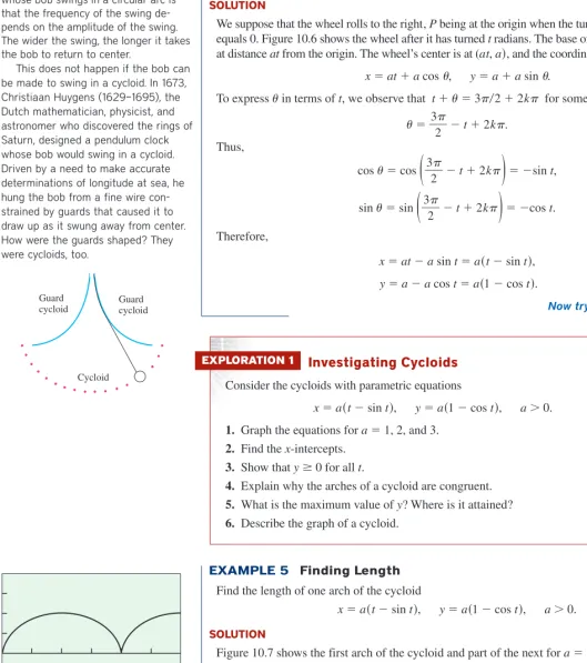
[image:5.684.40.569.97.693.2]

SOLUTION

Figure 10.7 shows the first arch of the cycloid and part of the next for

a

1. In

Explo-ration 1 you found that the

x

-intercepts occur at

t

equal to multiples of 2

and that the

arches are congruent.

The length of the first arch is

2

0

(

d

d

x

t

)

2

(

d

d

y

t

)

2

dt.

continued

Huygens’s Clock

The problem with a pendulum clock whose bob swings in a circular arc is that the frequency of the swing de-pends on the amplitude of the swing. The wider the swing, the longer it takes the bob to return to center.

This does not happen if the bob can be made to swing in a cycloid. In 1673, Christiaan Huygens (1629–1695), the Dutch mathematician, physicist, and astronomer who discovered the rings of Saturn, designed a pendulum clock whose bob would swing in a cycloid. Driven by a need to make accurate determinations of longitude at sea, he hung the bob from a fine wire con-strained by guards that caused it to draw up as it swung away from center. How were the guards shaped? They were cycloids, too.

Guard

cycloid Guardcycloid

Cycloid

[0, 3p] by [–2, 4]

Figure 10.7 The graph of the cycloid

Section 10.1 Parametric Functions 535

We have

(

d

d

x

t

)

2

a

1

cos

t

2

_a

2

₁

_{2 cos}

_t

_cos

2

_t

(

d

_d

y

_t

)

2

a

sin

t

2

_a

2

_sin

2

_t

(

d

_d

x

_t

)

2

(

d

_d

y

_t

)

2

a

2

2

c

o

s

t

.

a0, sin2_tcos2_t1

Therefore,

2

0

(

d

_d

x

_t

)

2

(

d

_d

y

_t

)

2

dt

a

2

0

2

2

c

o

s

t

dt

8

a.

Using NINT

The length of one arch of the cycloid is 8

a.

Now try Exercise 43.

Use algebra or a trig identity to write an equation relating xand y.

1. xt1 and y2t3 y2x1

2. x3t and y54t3_{3 y2x}3₃

3.xsin t and ycos t x2_y2₁

4.xsin t cos t and ysin(2t) y2x

5.xtan and ysec y2_1x2

Quick Review 10.1

(For help, go to Appendix A.1.)

6.xcsc and ycot x2_1y2

7.xcos and ycos(2) y2x2₁

8.xsin and ycos(2) y12x2

9.xcos and ysin (0 ) y1x2

10.xcos and ysin (2) y 1x2

Section 10.1 Exercises

In Exercises 1–6, sketch the parametric curves and identify those which define yas a function of x. In each case, eliminate the parame-ter to find an equation that relates xand ydirectly.

1.x2t3 and y4t3 for tin the interval [0, 3]

2. xt2 and y t

4 5

for tin the interval [3, 11]

3.xtan t and ysec t for tin the interval [0,

4]

4. xsin t and y2 cos t for tin the interval [0,]

5. xsin t and ycos(2t) for tin the interval [0, 2]

6.xsin 6t and y2t for tin the interval [0,

2] In Exercises 7–16, find (a) dy

dxand (b) d2_y

_dx2_{in terms of t.}

7.x4 sint, y2 cost 8. xcost, y3cost

9. x t1, y3t 10. x1

t, y 2lnt

11.xt2_{3t, yt}3 _{12. xt}2_{t, yt}2_t

13. xtan t, ysec t 14.x2cos t, ycos(2t)

15. xln(2t), yln(3t)4

16. xln(5t), ye5t

In Exercises 17–22,

(a) sketch the curve over the given t-interval, indicating the direction in which it is traced,

(b) identify the requested point, and

(c) justify that you have found the requested point by analyzing an appropriate derivative.

17. xt1, yt2_{t, 2t 2 Lowest point}

18. xt2_{2t, yt}2_{2t3, 2t 3 Leftmost point}

19. x2 sin t, ycos t, 0t Rightmost point

20. xtan t, y2 sec t, 1t 1 Lowest point

21. x2 sin t, ycos(2t), 1.5t 4.5 Highest point

22. xln(5t), yln(4t2_{), 0t 10 Rightmost point}

In Exercises 23–26, find the points at which the tangent line to the curve is (a) horizontal or (b) vertical.

23. x2cost, y 1sint

24. xsect, ytant 25. x2t, yt3_4t

26. x 23 cost, y13 sint

7. (a)1

2tan t (b) 1 8sec3t 8. (a)3 (b)0

9. (a)

33_t (b) t3/2

3

10. (a)t (b)t2

11. (a)

2t

3

t2

3

(b)6

(2

t2 t

1 3 8 )3

t

12. (a)2

2

t t

1 1

(b)

(2t

4 1)3

13. (a)sin t (b)cos3_t 14. (a)2 cos t (b)1

15. (a)4 (b)0

16. (a)5t e5t _(b)25t2_e5t_{5t e}5t

23. (a)(2, 0) and (2,2) (b)(1,1) and (3,1)

24. (a)Nowhere (b)(1, 0) and (1, 0)

26. (a)(2, 4) and (2,2)

(b)(1, 1) and (5, 1)

25. (a)At t 2 3

, or (0.845,3.079) and (3.155, 3.079) (b)Nowhere

In Exercises 27–34, find the length of the curve. (For an algebraic challenge, try evaluating the integrals without a calculator.)

27. xcos t, ysin t, 0t 2 2

28. x3 sin t, y3 cos t, 0t 3

29. x8 cost8tsint, y8 sint8tcost, 0t

2 2

30. x2 cos3_{t, y2 sin}3_{t, 0t 2 12}

31. x 2t

3 332

, yt t

2

2

, 0t3 21/2

32. x (8t

12 8)32

, yt2_{t, 0t 2 10}

33. x 1

3t

3_{, y} 1

2t

2_{, 0t1} 22

3

1

0.609

34. xlnsecttantsint, ycost, 0t

3 ln 2

35. Length is Independent of Parametrization To illustrate

the fact that the numbers we get for length do not usually depend on the way we parametrize our curves, calculate the length of the semicircle y1x2_{with these two different}

parametrizations.

(a) xcos 2t, ysin 2t, 0t

2

(b) xsint, ycost, 1

2t1

2

36. Perimeter of an Ellipse Find the length of the ellipse

x3 cost, y4 sint, 0t2.

37. Cartesian Length Formula The graph of a function yfx

over an interval a, bautomatically has the parametrization

xx, yfx, axb.

The parameter in this case is xitself. Show that for this parametrization, the length formula

L

b

a

(

d_dx_t

)

2

(

d_dy_t

)

2

dt

reduces to the Cartesian formula

L

b

a

1

(

d

d y x

)

2 dx

derived in Section 7.4. Just substitute xfor tand note that dx/dx1.

38. (Continuation of Exercise 37) Show that the Cartesian

formula

L

d

c

1

(

d

d x y

)

2 dy

for the length of the curve xgy, cyd, from Section 7.4 is a special case of the parametric length formula

L

b

a

(

d_dx_t

)

2

(

d_dy_t

)

2

dt.

Exercises 39 and 40 refer to the region bounded by the x-axis and one arch of the cycloid

xatsint, ya1cost

that is shaded in the figure shown at the top of the next column.

39. Find the area of the shaded region. (Hint: dxdx

dtdt) 3a2

40. Find the volume swept out by revolving the region about the

x-axis. (Hint: dVy2_dxy2_dx

_{dtdt) 5}2_a3

41. Curtate Cycloid Modify Example 4 slightly to find the

parametric equations for the motion of a point in the interiorof a wheel of radius aas the wheel rolls along the horizontal line without slipping. Assume that the point is at distance bfrom the center of the wheel, where 0 ba. This curve, known as a

curtate cycloid,has been used by artisans in designing the arches of violins (Source:mathworld.wolfram.com).

42. Prolate Cycloid Modify Example 4 slightly to find the

parametric equations for the motion of a point on the exteriorof a wheel of radius aas the wheel rolls along the horizontal line without slipping. Assume that the point is at distance bfrom the center of the wheel, where ab2a. This curve, known as a

prolate cycloid,is traced out by a point on the outer edge of a train’s flanged wheel as the train moves along a track. (If you graph a prolate cycloid, you can see why they say that there is always part of a forward-moving train that is moving backwards!)

43. Arc Length Find the length of one arch (that is, the curve

over one period) of the curtate cycloid defined parametrically by

x3t2 sin tand y3 2 cos t. 21.010

44. Arc Length Find the length of one arch (that is, the curve

over one period) of the prolate cycloid defined parametrically by

x2t3 sin tand y2 3 cos t. 21.010

Standardized Test Questions

You should solve the following problems without using a graphing calculator.

45. True or False In a parametrization, if xis a continuous function of tand yis a continuous function of t, then yis a continuous function of x. Justify your answer.

46. True or False If fis a function with domain all real numbers, then the graph of fcan be defined parametrically by xt and

yf(t) for t . Justify your answer.

47. Multiple Choice For which of the following parametrizations of the unit circle will the circle be traversed clockwise? B

(A) xcos t, ysin t, 0t2

(B) xsin t, ycos t, 0t2

(C) x cos t, y sin t, 0t2

(D) x sin t, ycos t, 0t2

(E) xsin t, y cos t, 0t2

2ap x

y

2a

22.103

38.Use the parametrization xg(y),yy,

cyd, substitute yfor tand note dy/dy1.

xatbsin tand yabcos t (0ab)

xatbsin tand yabcos t (ab2a)

45.False. Indeed,ymay not even be a function of x. (See Example 1.)

Section 10.1 Parametric Functions 537

48. Multiple Choice A parametric curve is defined by xsin t

and ycsc t for 0 t

2. This curve is C

(A) increasing and concave up.

(B) increasing and concave down.

(C) decreasing and concave up.

(D) decreasing and concave down.

(E) decreasing with a point of inflection.

49. Multiple Choice The parametric curve defined by xln(t),

ytfor t 0 is identical to the graph of the function C

(A) yln x for all real x.

(B) ylnx _{for x0.}

(C) yex _{for all real x.}

(D) yex _{for x0.}

(E) yln(ex_{) for x0.}

50. Multiple Choice The curve parametrized by

x6 sin t3 sin(7t) and y6 cos t3 cos(7t), as shown in the diagram below, is traversed exactly once as t

increases from 0 to 2. The total length of the curve is given by

(A)

2

0

(6 sin

t

3 s

in(7t)) 2₍₆

cos t

3 cos(7

t))2_dt

(B)

2

0

(6 cos

t

3 c

os(7t)) 2₍₆

sin t

3 sin (7

t))2_dt

(C)

2

0

(6 cos

t

21

cos(7t)) 2

(6 sin

t

21

sin(7t))

2_dt

(D)

2

0

(6 cos

t

21

cos(7t)) 2

(6 si

n t21 sin(7

t

))2_dt

(E)

2

0 7

(6 cos

t

3 cos (7

t)) 2₍₆

sin t

3 sin (3

t))2_dt

the string is tangent to the circle at Q, and tis the radian measure of the angle from the positive x-axis to the segment OQ.

(a)Derive parametric equations for the involute by expressing the coordinates xand yof Pin terms of tfor t0. xcos t

(b)Find the length of the involute for 0t2. ₂2

52. (Continuation of Exercise 51) Repeat Exercise 51 using the

circle of radius acentered at the origin, x2_y2_a2_.

In Exercises 53–56, a projectile is launched over horizontal ground at an angle with the horizontal and with initial velocity v₀ft

sec. Its path is given by the parametric equations

xv₀cost, yv₀sint16t2_.

(a)Find the length of the path traveled by the projectile.

(b)Estimate the maximum height of the projectile.

53. 20°, v₀150 54. 30°, v₀150

55. 60°, v₀150 56. 90°, v₀150

Extending the Ideas

If dx

dtand dy

dtare continuous, the parametric curve defined by (x(t),y(t)) for a t bis called smooth. If the curve is traversed exactly once as tincreases from ato b, and if yis a positive function of x, then the curve can be revolved about the x-axis to form a solid of revolution (see Section 7.3). The surface areaof such a solid is given by

S

b

a

2y

(

d d x t

)

2

(

d_dy_t

)

2

dt.

Apply this formula in Exercises 57–60 to find the surface area when the parametric curve is revolved about the x-axis.

57. xcos t, y2sin t, 0t2 82

58. x2t, y(2

3)t32_{, 0t2 14.214}

59. xt2_{2, yt1, 0t3 178.561}

60. xln(sec ttan t)sin t, ycos t, 0t

3 10

–10 –10

2 10

2 –2

x y

x y

O t

P(x, y)

(1, 0) String

1 Q

Explorations

51. Group Activity Involute of a Circle If a string wound around a fixed circle is unwound while being held taut in the plane of the circle, its end Ptraces an involute of the circle as suggested by the diagram below. In the diagram, the circle is the unit circle in the xy-plane, and the initial position of the tracing point is the point 1, 0on the x-axis. The unwound portion of

D

tsin t, ysin ttcos t

(a)xa(cos ttsin t),ya(sin ttcos t) (b)2a2

(a) 461.749 ft (b) 41.125 ft

(a) 840.421 ft (b)16,875/64263.672 ft (a)703.125 ft

(b)5625/16351.5625 ft

(a) 641.236 ft (b)5625/6487.891 ft

Vectors in the Plane

Two-Dimensional Vectors

When an object moves

along a straight line

, its velocity can be determined by a single

num-ber that represents both magnitude and direction (forward if the numnum-ber is positive, backward

if it is negative). The speed of an object moving on a path

in a plane

can still be represented by

a number, but how can we represent its direction when there are an infinite number of

direc-tions possible? Fortunately, we can represent both magnitude and direction with just two

numbers, just as we can represent any point in the plane with just two coordinates (which is

possible essentially for the same reason). This representation is what two-dimensional vectors

were designed to do.

While the pair (

a

,

b

) determines a point in the plane, it also determines a

directed line

segment

(or

arrow

) with its tail at the origin and its head at (

a

,

b

) (Figure 10.8). The length of

this arrow represents magnitude, while the direction in which it points represents direction. In

this way, the ordered pair (

a

,

b

) represents a mathematical object with both magnitude and

di-rection, called the

position vector of (

a

,

b

)

.

10.2

What you’ll learn about

• Two-Dimensional Vectors

• Vector Operations

• Modeling Planar Motion

• Velocity, Acceleration, and

Speed

• Displacement and Distance

Traveled

. . . and why

The jump from one to two

dimen-sions (and eventually higher) is

easier than one might think,

thanks to the mathematics of

vectors.

(a, b)

a, b y

x O

O

(a, b) y

x

Figure 10.8 The point represents the ordered pair (a,b). The arrow (directed line segment) represents the vector a,b.

The distance formula in the plane gives a simple computational formula for magnitude.

DEFINITION

Two-Dimensional Vector

A

two-dimensional vector v

is an ordered pair of real numbers, denoted in

component

form

as

a

,

b

. The numbers

a

and

b

are the

components

of the vector

v

. The

standard

representation

of the vector

a

,

b

is the arrow from the origin to the point (

a

,

b

).

The

magnitude

(or

absolute value

) of

v

, denoted

v

, is the length of the arrow, and the

direction of v

is the direction in which the arrow is pointing. The vector

0

0, 0

,

called the

zero vector

, has zero length and no direction.

Direction can be quantified in several ways; for example, navigators use bearings from

compass points. The simplest choice for us is to measure direction as we do with the

trigonometric functions, using the usual position angle formed with the positive

x

-axis as

the initial ray and the vector as the terminal ray. In this way, every nonzero vector

deter-mines a unique

direction angle

satisfying (in degrees) 0

360 or (in radians)

0

2

. (See Figure 10.10 for an example.)

Magnitude of a Vector

[image:10.684.48.196.52.169.2]

Section 10.2 Vectors in the Plane 539

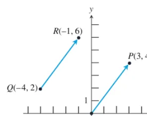
Figure 10.9 The arrows QRand OP

both represent the vector 3, 4, as would any arrow with the same length pointing in the same direction. Such arrows are called

equivalent.

P(3, 4)

O R(–1, 6)

Q(–4, 2)

1 1

x y

Head Minus Tail (HMT) Rule

If an arrow has initial point (

x

₁

,

y

₁

) and terminal point (

x

₂

,

y

₂

), it represents the

vector

x

₂

x

₁

,

y

₂

y

₁

.

EXAMPLE 1

Finding Magnitude and Direction

Find the magnitude and the direction angle

of the vector

v

1,

3

(Figure 10.10).

SOLUTION

The magnitude of

v

is

v

(

1

0)

2

₍

₃

₀₎

2

_{2. Using triangle ratios, we see}

that the direction angle

satisfies cos

1

2 and sin

3

2, so

120º or 2

3

radians.

Now try Exercise 5.

EXAMPLE 2

Finding Component Form

Find the component form of a vector with magnitude 3 and direction angle 40º.

SOLUTION

The components of the vector, found trigonometrically, are

x

3 cos 40º and

y

3 sin 40º

(Figure 10.11).

The vector is

3 cos 40º, 3 sin 40º

2.298, 1.928

.

Now try Exercise 13.

Vector Operations

The algebra of vectors sometimes involves working with vectors and numbers at the same

time. In this context, we refer to the numbers as

scalars

. The two most basic algebraic

opera-tions involving vectors are

vector addition

(adding a vector to a vector) and

scalar

multiplica-tion

(multiplying a vector by a number). Both operations are easily represented geometrically.

v

(

–1, √−3

)

u

–2

–2 2

2 x

[image:10.684.54.190.410.539.2]

y

Figure 10.10 The vector vin Example 1 is represented by an arrow from the origin to the point

1,3.

Why Not Use Slope for Direction?

Notice that slopeis inadequate for de-termining the direction of a vector, since two vectors with the same slope could be pointing in opposite directions. More-over, vectors are still useful in dimen-sions higher than 2, while slope is not.

y = 3 sin 40˚ 40˚

3

x = 3 cos 40˚

–1

3 x y

Figure 10.11 The vector in Example 2 is represented by an arrow from the origin to the point (3 cos 40º, 3 sin 40º).

Direction Angle of a Vector

The

direction angle

of a nonzero vector

v

is the smallest nonnegative angle

formed with the positive

x

-axis as the initial ray and the standard representation

of

v

as the terminal ray.

This textbook uses boldface variables to represent vectors (for example,

u

and

v

) to

dis-tinguish them from numbers. In handwritten form it is customary to disdis-tinguish vector

variables by arrows (for example,

u

and

v

). We also use angled brackets to distinguish a

vector

x

,

y

from a point (

x

,

y

) in the plane, although it is not uncommon to see (

x

,

y

)

used for both, especially in handwritten form.

It is often convenient in applications to represent vectors with arrows that begin at points

other than the origin. The important thing to remember is that

any two arrows with the same

length and pointing in the same direction represent the same vector

. In Figure 10.9, for

ex-ample, the vector

3, 4

is shown represented by

QR

, an arrow with

initial point

Q

and

terminal point

R

, as well as by its standard representation

O

OP

. Two arrows that represent

the same vector are said to be

equivalent

.

The quick way to associate arrows with the vectors they represent is to use the following

rule.

The vector

v

v

is a vector of magnitude 1, called a

unit vector

. Its component form is

cos

, sin

, where

is the direction angle of

v

. For this reason,

v

v

is sometimes called

the

direction vector

of

v

.

The sum of two vectors

u

and

v

can be represented geometrically by arrows in two ways.

In the

tail-to-head representation

, the arrow from the origin to (

u

₁

,

u

₂

) is the standard

repre-sentation of

u

, the arrow from (

u

₁

,

u

₂

) to (

u

₁

v

₁

,

u

₂

v

₂

,) represents

v

(as you can verify by

the HMT Rule), and the arrow from the origin to (

u

₁

v

₁

,

u

₂

v

₂

) then is the standard

repre-sentation of

u

v

(Figure 10.12a).

In the

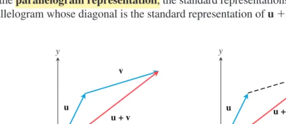
parallelogram representation

, the standard representations of

u

and

v

determine

a parallelogram whose diagonal is the standard representation of

u

v

(Figure 10.12b).

v

u _{u + v}

v u

(a) (b)

u + v

x y

[image:11.684.207.566.57.301.2]

x y

Figure 10.12 Two ways to represent vector addition geometrically: (a) tail-to-head and (b) parallelogram.

–2 u

u u

2 u

1 _ 2

Figure 10.13 Representations of uand several scalar multiples of u.

The product

k

u

of the scalar

k

and the vector

u

can be represented by a stretch (or shrink)

of

u

by a factor of

k

. If

k

0, then

k

u

points in the same direction as

u

; if

k

0, then

k

u

points in the opposite direction (Figure 10.13).

EXAMPLE 3

Performing Operations on Vectors

Let

u

1, 3

and

v

4, 7

. Find the following.

(a)

2

u

3

v

(b) u

v

(c)

1

2

u

SOLUTION

(a)

2

u

3

v

2

1, 3

3

4, 7

2

1

3

4

, 2

3

3

7

10, 27

continued

DEFINITION

Vector Addition and Scalar Multiplication

Let

u

u

₁

,

u

₂

and

v

v

₁

,

v

₂

be vectors and let

k

be a real number (scalar).

The

sum

(or

resultant

)

of the vectors u and v

is the vector

u

v

u

₁

v

₁

,

u

₂

v

₂

.

The

product of the scalar

k

and the vector u

is

k

u

k

u

₁

,

u

₂

ku

₁

,

ku

₂

.

The

opposite of a vector v

is

v

(

1)

v

. We define vector subtraction by

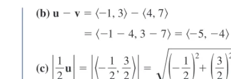
[image:11.684.255.534.375.496.2]

(b) u

v

1, 3

4, 7

1

4, 3

7

5,

4

(c)

1

2

u

1

2

,

3

2

(

1

2

)

2

(

3

2

)

2

1

2

1

0

Now try Exercise 21.

Vector operations have many of the properties of their real-number counterparts.

Section 10.2 Vectors in the Plane 541

Modeling Planar Motion

Although vectors are used in many other physical applications, our primary reason for

introducing them into this course is to model the motion of objects moving in a

coordi-nate plane. You may have seen vector problems of the following type in a physics or

mechanics course.

EXAMPLE 4

Finding Ground Speed and Direction

A Boeing

®

₇₂₇

®

_{airplane, flying due east at 500 mph in still air, encounters a 70-mph tail}

wind acting in the direction 60º north of east. The airplane holds its compass heading due

east but, because of the wind, acquires a new ground speed and direction. What are they?

SOLUTION

If

u

the velocity of the airplane alone and

v

the velocity of the tail wind, then

u

500 and

v

70 ( Figure 10.14).

We need to find the magnitude and direction of the

resultant vector

u

v

. If we let the

positive

x

-axis represent east and the positive

y

-axis represent north, then the

compo-nent forms of

u

and

v

are

u

500, 0

and

v

70 cos 60º, 70 sin 60º

35, 35

3

.

Therefore,

u

v

535, 35

3

,

u

v

5

3

5

2

₃

₅

₃

2

_538.4,

and

tan

1

35

5

35

3

6.5º.

Interpret

The new ground speed of the airplane is about 538.4 mph, and its new

direction is about 6.5º north of east.

Now try Exercise 25.

Properties of Vector Operations

Let

u

,

v

,

w

be vectors and

a

,

b

be scalars.

1. u

v

v

u

2.

u

v

w

u

v

w

3. u

0

u

4. u

u

0

5.

0

u

0

6.

1

u

u

7.

a

b

u

ab

u

8.

a

u

v

a

u

a

v

9.

a

b

u

a

u

b

u

E N

u v

u + v 30

˚

70

500

[image:12.684.213.439.51.128.2]

NOT TO SCALE

Figure 10.14 Vectors representing the velocities of the airplane and tail wind in Example 4.

Recall that if the position

x

of an object moving along a line is given as a function of time

t

,

then the velocity of the object is

dx

dt

and the acceleration of the object is

d

2

_x

_dt

2

_{. It is}

al-most as simple to relate position, velocity, and acceleration for an object moving in the

plane, because we can model those functions with vectors and treat

the components of the

vectors as separate linear models

. Example 5 shows how simple this modeling actually is.

EXAMPLE 5

Doing Calculus Componentwise

A particle moves in the plane so that its position at any time

t

0 is given by (sin

t

,

t

2

_2).

(a)

Find the position vector of the particle at time

t

.

(b)

Find the velocity vector of the particle at time

t

.

(c)

Find the acceleration of the particle at time

t

.

(d)

Describe the position and motion of the particle at time

t

6.

SOLUTION

(a)

The position vector, which has the same components as the position point, is

sin

t

,

t

2

₂

_.

In fact, it could also be represented as (sin

t

,

t

2

_{2), since the context would identify it as}

a vector.

(b)

Differentiate each component of the position vector to get

cos

t

,

t

.

(c)

Differentiate each component of the velocity vector to get

sin

t

, 1

.

(d)

The particle is at the point (sin 6, 18), with velocity

cos 6, 6

and acceleration

sin 6, 1

.

You can graph the path of this particle parametrically, letting

x

sin(

t

) and

y

t

2

_{2. In}

Figure 10.15 we show the path of the particle from

t

0 to

t

6. The red arrow at the

point (sin 6, 18) represents the velocity vector (cos 6, 6). It shows both the magnitude and

direction of the velocity at that moment in time.

Now try Exercise 31.

Velocity, Acceleration, and Speed

We are now ready to give some definitions.

EXAMPLE 6

Studying Planar Motion

A particle moves in the plane with position vector

r

(

t

)

sin (3

t

), cos (5

t

)

. Find the

velocity and acceleration vectors and determine the path of the particle.

continued

[–2, 2] by [0, 25]

0 ≤ t ≤ 6

cos 6 6

Figure 10.15 The path of the particle in Example 5 from t0 to t6. The red arrow shows the velocity vector at t6.

A Word About Differentiability

Our definitions can be expanded to a

calculus of vectors, in which (for ex-ample) dv

dta(t), but it is not our in-tention to get into that here. We have therefore finessed the fine point of vec-tor differentiability by requiring the path of our particle to be “smooth.” The path can have vertical tangents, fail the vertical line test, and loop back on itself, but corners and cusps are still problematic.

DEFINITIONS

Velocity, Speed, Acceleration, and Direction

of Motion

Suppose a particle moves along a smooth curve in the plane so that its position at

any time

t

is (

x

(

t

)),

y

(

t

), where

x

and

y

are differentiable functions of

t

.

1.

The particle’s

position vector

is

r

(

t

)

x

(

t

),

y

(

t

)

.

2.

The particle’s

velocity vector

is

v

(

t

)

d

d

x

t

,

d

d

y

t

.

3.

The particle’s

speed

is the magnitude of

v

, denoted

v

. Speed is a

scalar

, not a

vector.

4.

The particle’s

acceleration vector

is

a

(

t

)

d

dt

2

_x

2

,

d

dt

2

_y

2

.

5.

The particle’s

direction of motion

is the

direction vector