www.biogeosciences.net/11/4077/2014/ doi:10.5194/bg-11-4077-2014
© Author(s) 2014. CC Attribution 3.0 License.
Strong sensitivity of Southern Ocean carbon uptake and nutrient
cycling to wind stirring
K. B. Rodgers1, O. Aumont2, S. E. Mikaloff Fletcher3, Y. Plancherel4, L. Bopp5, C. de Boyer Montégut6, D. Iudicone7, R. F. Keeling8, G. Madec9,10, and R. Wanninkhof11
1AOS Program, Princeton University, Princeton, NJ, USA 2IRD, Plouzané, France
3NIWA, Wellington, New Zealand
4Department of Earth Sciences, University of Oxford, Oxford, UK 5LSCE, IPSL, CNRS, CEA, UVSQ, Gif-sur-Yvette, France
6IFREMER, Centre de Brest, Laboratoire d’Océanographie Spatiale, Plouzané, France 7Stazione Zoologica Anton Dohrn, Naples, Italy
8Scripps Institute of Oceanography, UCSD, San Diego, CA, USA 9LOCEAN, CNRS, IRD, UPMC, MNHN, IPSL, Paris, France 10National Oceanography Centre, Southampton, UK
11NOAA-AOML, Miami, FL, USA
Correspondence to: K. B. Rodgers (krodgers@princeton.edu)
Received: 28 July 2013 – Published in Biogeosciences Discuss.: 13 September 2013 Revised: 13 June 2014 – Accepted: 19 June 2014 – Published: 1 August 2014
Abstract. Here we test the hypothesis that winds have an im-portant role in determining the rate of exchange of CO2 be-tween the atmosphere and ocean through wind stirring over the Southern Ocean. This is tested with a sensitivity study us-ing an ad hoc parameterization of wind stirrus-ing in an ocean carbon cycle model, where the objective is to identify the way in which perturbations to the vertical density structure of the planetary boundary in the ocean impacts the carbon cycle and ocean biogeochemistry.
Wind stirring leads to reduced uptake of CO2by the South-ern Ocean over the period 2000–2006, with a relative reduc-tion with wind stirring on the order of 0.9 Pg C yr−1over the region south of 45◦S. This impacts not only the mean carbon uptake, but also the phasing of the seasonal cycle of carbon and other ocean biogeochemical tracers. Enhanced wind stir-ring delays the seasonal onset of stratification, and this has large impacts on both entrainment and the biological pump. It is also found that there is a strong reduction on the order of 25–30 % in the concentrations of NO3exported in Sub-antarctic Mode Water (SAMW) to wind stirring. This finds expression not only locally over the Southern Ocean, but also over larger scales through the impact on advected
nutri-ents. In summary, the large sensitivity identified with the ad hoc wind stirring parameterization offers support for the im-portance of wind stirring for global ocean biogeochemistry through its impact over the Southern Ocean.
1 Introduction
thoroughly explored. Our main focus is to conduct such an analysis for the case of carbon over the Southern Ocean, but also to give more general consideration to other tracers re-lated to ocean biogeochemistry. This is considered within the context of the full seasonal cycle over the Southern Ocean, and the implications for trends in carbon uptake are explored. There is widespread interest in understanding the way in which surface atmospheric winds contribute to the partition-ing of CO2between the oceanic and atmospheric reservoirs. Surface winds may impact the ocean carbon cycle in three ways:
1. through wind-driven microturbulence at the air–sea in-terface that controls the gas exchange velocity;
2. through wind-driven meridional overturning and water mass transformations, as impacted by large-scale inter-actions with the atmosphere, including the net transfer of momentum and buoyancy to the ocean over large scales;
3. through wind-driven stirring and the transfer of energy over the planetary boundary layer of the ocean (within the mixed layer and below) through shear-induced tur-bulence.
The issue of air–sea gas exchange has been and continues to be the focus of extensive research, including the develop-ment of gas exchange parameterizations for use with models (Wanninkhof, 1992; see Wanninkhof et al., 2009 for a more extensive overview). The magnitude of the derived piston ve-locity exerts a major control on seasonal variations in air–sea CO2 fluxes but has less influence on the long-term uptake of CO2, which is mainly controlled by circulation and mix-ing within the ocean (Bolin and Eriksson, 1958; Sarmiento et al., 1992). Models show instead much greater sensitivi-ties to changes in the physical transport and mixing param-eterizations, particularly in the Southern Ocean (Mignone et al., 2006). A number of studies (Wyrtki, 1961; Toggweiler and Samuels, 1993; Gnanadesikan, 1999) have established a central role for winds over the Southern Ocean in deter-mining the overturning circulation of the global ocean and therefore ocean carbon cycling. More recent work with eddy-permitting models (Hallberg and Gnanadesikan, 2006) and observationally based analyses (Böning et al., 2008) has also drawn attention to the importance of geostrophic turbulence (ocean eddies) in modulating the response of the overturning circulation to perturbations in surface winds. The study of the implications of geostrophic turbulence for the Southern Ocean carbon cycle is an active area of research (Ito et al., 2010).
The issue of shear-induced turbulence and wind stirring has received far less attention to date and it is the focus of this study. The mechanical input of energy from the winds into the upper ocean and the subsequent dissipation through
shear-induced mixing may play a role in determining sum-mer mixed-layer depths. This is likely to be of particular im-portance over the Southern Ocean, where 50 m mixed-layer depths are sustained through summer under the influence of the maximum westerlies between 50–60◦S, with no consen-sus yet on the mechanisms that consen-sustain this phenomenon. The two main mechanisms for wind stirring over this region may be expected to be upper-ocean near-inertial oscillations (Jochum et al., 2013) and ocean swells and waves (Qiao et al., 2004; Huang et al., 2012; Huang and Qiao, 2010). The relative importance of these mechanisms remains unknown. Importantly, these two mechanisms result in a net erosion of stratification, and they add potential energy to the upper ocean. As such, their impact in stratification stands in marked contrast to that of mesoscale eddies, which remove potential energy from the ocean. Thus, shear-induced turbulence and geostrophic turbulence should have opposing effects on cli-matological mixed-layer depths averaged over particular sea-sons.
The current generation of coupled and ocean-only mod-els tends to exhibit shallow summer mixed-layer biases over the Southern Ocean (Huang et al., 2012) and excessive strat-ification at the base of the mixed layer. It has been shown that Southern Ocean winds are typically too weak and too far equatorward in coupled models (Fyfe and Saenko, 2006), which may explain some of the mixed-layer bias in these models. Nonetheless, Southern Ocean summer mixed lay-ers are also too shallow in ocean-only models forced with observed atmospheric winds and buoyancy fluxes, indicat-ing that important physical processes responsible for upper-ocean mixing are missing from current model formulations.
The degree to which the shallow summer mixed-layer bias affects the ability of models to correctly simulate uptake and storage patterns of carbon and heat is not clear but differ-ent argumdiffer-ents suggest it is not negligible. First, the depth of the actively mixed layer in the upper ocean defines the total light available to phytoplankton (de Baar et al., 2005) and thus affects models’ ability to correctly simulate the biologi-cal response to iron supply in the Southern Ocean, inducing an error in simulations of the biological pump. More gener-ally, the misrepresentation of seasonal mixed-layer dynamics affects the overall biogeochemical landscape in the Southern Ocean (Marinov et al., 2006). Since the Southern Ocean ex-ports nutrients that fuel a large part of low latitude productiv-ity (Sarmiento et al., 2004), these regional errors that affect the processes determining the distribution and seasonal cy-cling of nutrients in the Southern Ocean can have long-range effects.
the physical environment, on local and global biogeochem-istry and on the overall ability of the Southern Ocean to main-tain its role as a region of intense heat and carbon uptake.
Here, an ad hoc wind stirring parameterization that al-lows energy from the winds to be input into the region be-low the base of the mixed layer was added to a global ocean biogeochemistry model in order to correct for the summer mixed-layer bias in the model and better represent summer mixed-layer dynamics. By contrasting two model runs, one with the ad hoc parameterization and a control run with-out, we evaluate the sensitivity of oceanic CO2uptake and ocean biogeochemistry to the imposed change in wind stir-ring. We show that accounting for the additional effect of wind stirring greatly reduces contemporary carbon uptake in the Southern Ocean. The reasons for this effect and its consequences on the geographical distribution of carbon and oxygen fluxes, mixed-layer depth, stratification, chlorophyll, and nutrients are investigated further, highlighting the impor-tance of wind stirring on the seasonal cycle of these proper-ties. Finally, given protected future changes in the intensity and frequency of storms (Wu et al., 2010), we consider our two simulations with and without wind stirring as represen-tative of two hypothetical climate states, one with low and one with high storminess. Furthermore, we question if in-creased storminess, as simulated by the added ad hoc param-eterization, has an effect on atmospheric CO2levels by im-pacting the oceanic carbon sink. Because terrestrial processes contribute to atmospheric CO2 variability, we rely here on the concept of atmospheric potential oxygen (APO) (Keeling and Schertz, 1992; Stephens et al., 1998), a tracer that is con-served with respect to the terrestrial biosphere and primarily reflects ocean fluxes. We show that a change in wind stirring manifests itself as a shift in the phasing of the seasonal APO cycle in the sub-polar Southern Hemisphere. If large enough, this shift should be detectable from the existing network of atmospheric monitoring stations.
2 Methods
2.1 General model description and experimental design The experiments are performed with the NEMO-PISCES model (Madec et al., 1998; Aumont and Bopp, 2006) in the global ORCA2 configuration of NEMO Version 3.2. Hori-zontal resolution is 2◦, increasing to approximately 1◦over
the Southern Ocean. Mesoscale eddies are parameterized with the scheme of Gent and McWilliams (1990). Vertical mixing in NEMO is achieved using the turbulence kinetic energy (TKE) parameterization of Blanke and Delecluse (1993), and the TKE parameterization includes a Langmuir cell parameterization (Axell, 2002).
The representation of light limitation in the evolution of the PISCES model used here has been modified relative to the version of PISCES described in Aumont and Bopp
(2006). The influence of light limitation on the growth rate of nanophytoplankton (µP) is modeled in this version of PISCES using a modified version of the Geider et al. (1998) formulation in which the nutrient co-limitation term and the dependence on temperature were removed in accordance with the findings by Li et al. (2010):
µP=µmax·
1−exp
−α·Chl
C · light
Pmax
, (1)
wherePmax is a constant that does not depend on temper-ature and nutrient limitation. Two simulations, WSTIR and CNTRL, are considered. WSTIR and CNTRL only differ in that an ad hoc parameterization (described below) for the ef-fect of wind stirring as a component of vertical mixing is used in WSTIR but not in CNTRL. Other than that, WSTIR and CNTRL have identical wind stresses and surface buoyancy boundary conditions, identical horizontal and vertical reso-lution, and identical biogeochemical and physical parameter settings. It is important to emphasize that the same param-eterization of gas exchange (Wanninkhof, 1992) with pre-cisely the same wind speeds is used for gas exchange for both WSTIR and CNTRL.
The initial state for temperature and salinity was taken from the World Ocean Atlas 2009 (WOA09) (Locarnini et al., 2010; Antonov et al., 2010), and the initial state for biogeochemistry was taken from a 5000-year pre-industrial spin-up of NEMO-PISCES. At the time of initialization for this study, the ocean was treated as being in a state of no mo-tion. This initial model state nominally corresponds to year 1864. The model was then forced at its upper surface using the DRAKKAR forcing set #4.1, or DFS4.1 (Brodeau et al., 2010), which is derived from the ERA-40 reanalysis prod-uct (Uppala et al., 2005) and has a temporal resolution of six hours. DFS4.1 spans years 1958–2006. The model was looped twice through repeating full DFS4.1 forcing fields cycles to reach year 1957 with atmospheric CO2 concen-trations increasing over this time. The two parallel simula-tions WSTIR and CNTRL were started in year 1958 as de-scribed above. As such, the same transient in atmospheric CO2boundary conditions is present in both simulations.
The question arises as to whether the time interval over which we considered the sensitivity to wind stirring (1958– 2006) is of sufficient duration to distinguish between spuri-ous signals associated with adjustments and the steady-state response of the Southern Ocean carbon cycle to our ad hoc wind stirring parameterization. Importantly, we are interested in both the adjustment period and the steady-state response of the system to the applied perturbation.
2.2 Ad hoc parameterization of wind stirring
this systematic bias, an ad hoc parameterization was intro-duced into the TKE vertical mixing scheme of Blanke and Delecluse (1993) within NEMO. The parameterization pre-sented here is not derived from theoretical considerations, but rather is meant to account for observed processes that affect the density structure of the ocean’s planetary boundary layer that are not explicitly captured by default in the TKE scheme. These processes are near-inertial oscillations (Jochum et al., 2013) and ocean swells and waves (Qiao et al., 2004; Huang et al., 2012; Huang and Qiao, 2010).
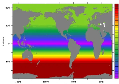
First, a vertical mixing-length scale hτ (Fig. 1) is
com-puted as a function of latitude (ϕ, units of latitude):
hτ=max(0.5,min(30,45·sin(ϕ)))∀ϕ≥0, (2) hτ=max(0.5,2·min(30,45·sin(ϕ)))∀ϕ <0.
Values for hτ vary from 0.5 m at the Equator to a
maxi-mum of 30 m in the high latitudes of the Northern Hemi-sphere and 60m in the Southern Ocean. The above definition of mixing length was tuned to achieve summer mixed-layer depths consistent with observations and that are also consis-tent with the wave-induced mixing-length scales reported by Qiao et al. (2004). During the tuning phase, vertical mixing-lengths spanning 30 m to 70 m were tried over the Southern Ocean, with 60 m providing the best match against observa-tional constraints.
The kinetic energy input to the ocean (S) imposed by the winds in the form of near-inertial oscillations, swell and waves is parameterized as follows:
S=εi·exp(−z hτ
)·(1−fi), (3)
wherezis the depth andεi(adjusted here to 0.07) is the
frac-tion of the kinetic energy imposed by wind stress as com-puted by the traditional TKE implementation of Blanke and Delecluse (1993) (TKEBD93). This value is similar to the scaling factorα=0.05 used by Jochum et al. (2013) to pa-rameterize the input of kinetic energy into the ocean due to near-inertial oscillations. The depth structure of the energy input function in the ocean interior is modeled using an expo-nential function that depends on the mixing-lengthhτ. This is modulated by the fractional sea-ice concentration (fi)as the influence of wind stress below sea ice is small. The overall kinetic energy input in WSTIR is obtained by summing the traditional TKE input obtained by the Blanke and Delecluse (1993) scheme and S:
TKEWSTIR=TKEBD93+S. (4)
As the magnitude of TKEBD93is much greater thanSin the mixed layer, the contribution ofS is relatively small there. The relative influence ofSis strongest just below the mixed layer at times and locations where the mixing-length hτ is
[image:4.612.310.547.64.231.2]greater than the mixed-layer depth generated by TKEBD93. In these locations,Serodes the stratification, thus contributing to deepening of the mixed layer.
Figure 1. The mixing-length scale over which the ad hoc wind
stir-ring parameterization is prescribed to act in the WSTIR simulation, in units of meters.
A number of observational products are available that pro-vide consistent views of seasonal variations in mixed-layer depths over the Southern Ocean (de Boyer Montégut et al., 2004; Dong et al., 2008; Huang et al., 2012). Here we choose to use a new 2013 update of the climatology of de Boyer Montégut et al. (2004), which has benefited from the large in-crease in Argo measurements over the last decade. The orig-inal release of this product, and the 2008 update, used a den-sity deviation from the surface of 0.03 kg m−3to characterize the base of the mixed layer. However, the increased quan-tity of Argo measurements now allows a density criterion of 0.01 kg m−3to be used, by overcoming signal-to-noise is-sues, and that is what we will use here. Given the relatively weak stratification of the Southern Ocean, this smaller cri-terion is appropriate for our analysis of seasonal variability in mixed-layer depths. Nevertheless, we will also consider the sensitivity of Southern Ocean mixed-layer depth (MLD) variations to the amplitude of this threshold.
2.3 Atmospheric potential oxygen: definition, simulation and observations
Observed variations in atmospheric CO2concentrations over seasonal to decadal timescales are difficult to interpret in terms of ocean processes as only a small fraction of the CO2 variability actually comes from the ocean. A much larger fraction of the variability in CO2is caused by exchanges with the land biosphere; this is true even in regions remote from direct land biospheric influences, such as the high latitudes of the Southern Hemisphere (e.g., Stephens et al., 2013). An at-mospheric constraint on oceanic processes can be derived by combining measurements of atmospheric CO2 and O2/N2 ratios to compute atmospheric potential oxygen (APO). APO is defined as follows:
In this expressionδO2/N2)is the ratio of O2to N2relative to the ratio in standard air and is referred to as having units of per meg (equivalent to per million). The emissions ratio of CO2to O2from terrestrial processes is typically 1.1 with only small deviations (Severinghaus et al., 2001). Since O2 comprises 20.94% of the atmosphere, a conversion factor of 1/0.2094=4.8 can be used to convert CO2 from units of ppm to units of per meg. APO is conserved with respect to the terrestrial biosphere, which causes compensating varia-tions inδ(O2/N2)and CO2. Much of the variability in APO over seasonal and shorter time scales reflects ocean fluxes (Keeling and Shertz, 1992; Stephens et al., 1998). In addi-tion, while physical and biological processes in the ocean of-ten have opposing effects on CO2, damping the atmospheric signal of these processes, they typically have additive effects on O2/N2. For example, summertime CO2 uptake repre-sents a balance of biologically driven uptake and thermally driven outgassing of CO2, while biological and thermal pro-cesses both lead to O2uptake.
High-frequency APO data are available down to the timescale of a week. Such high-frequency data are not avail-able for pCO2, for which there is also a well-known lack of both winter and summer measurements. APO also stands in contrast to remotely sensed ocean color products, whose temporal sampling can be strongly affected by cloud cover. Although APO data are only available for specific sites, these are atmospheric observations and they represent large well-mixed air masses that integrate surface processes over large parts of the Southern Ocean. The APO data from the Scripps network used in this study are described in detail in Hamme and Keeling (2008) and Keeling and Manning (2013).
In order to investigate the effect of the wind stirring param-eterization on APO, daily mean air–sea fluxes of O2, CO2, and heat from the WSTIR and CNTRL ocean simulations are used as lower boundary conditions in a three-dimensional at-mospheric transport model, Tracer Model Version 3 (TM3) (Heimann and Körner, 2003). Since the air–sea flux of N2is not modeled explicitly in NEMO-PISCES but is needed to simulate APO, the air–sea fluxes of N2are calculated from the heat fluxes following the formulation of Keeling and Peng (1995) using the temperature-dependent N2solubility of Weiss (1970).
TM3 is an offline model driven by the National Centers for Environmental Prediction (NCEP) reanalysis winds (Kalnay et al., 1996). The fine-grid version used here has a reso-lution of ∼3.8◦×5◦ with 19 vertical levels. TM3 is well
documented and has been included in many model inter-comparisons studies (e.g., Denning et al., 1999; Gurney et al., 2003), and compares well with other models when evaluated against aircraft data (Stephens et al., 2007). TM3 was run from 1990 to 2005 but only years 1994–2005 are analyzed to account for spin-up effects of the atmospheric model.
It is important to consider whether the inconsistency be-tween the ocean forcing reanalysis product (DRAKKAR) and the atmospheric transport fields used for APO (NCEP)
can be expected to impact our scientific results or interpre-tations. Our primary interest with these simulations is to use the seasonal behavior of APO to evaluate the two versions of the NEMO model. Blaine (2005) compared APO simu-lations from a suite of ten different atmospheric transport models using the same air–sea fluxes as boundary conditions, with some of the transport models driven by NCEP and some driven by ERA-40. For the high latitude Southern Ocean sta-tions, the atmospheric transport models simulated slightly different seasonal amplitudes, but were in good agreement regarding the seasonal cycle.
We also account for small variations in APO caused by fossil fuel burning. Fossil fuel emissions were distributed spatially according to the 1995 Carbon Dioxide Information Analysis Center (CDIAC) fossil fuel emissions map (Mar-land et al., 1998). The spatial distribution was then scaled for emissions for specific years (Boden et al., 2012). O2 con-sumed by fossil fuels was calculated simply by using a sim-ple combustion ratio of 1.4 moles of O2 for every mole of CO2(Keeling et al., 1998; Marland et al., 2003). Spatial and temporal variations of the O2/CO2 combustion ratio aris-ing from differences in fuel types are not considered, but this omission is unlikely to be problematic for our analysis and interpretation of the seasonal APO signal.
3 Results
3.1 Wind stirring, mixed-layer depths, and stratification
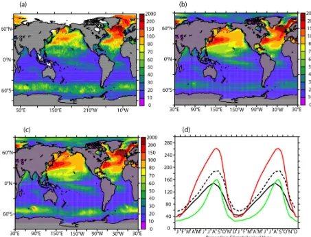
The 2014 update of the mixed-layer depth product of de Boyer Montégut et al. (2004) shows austral summer mixed layer depth on the order of 50 m (January) and austral win-ter mixed layer depth on the order of 150 m (October) in the latitude band 50–60◦S, the region under the maximum west-erlies (Fig. 2a, solid black line in Fig. 2d). Austral summer mixed-layer depths for CNTRL are consistently too shallow in the Southern Ocean (Fig. 2b), with summer mixed layer depths having maximum values on the order of only 20 m (Fig. 2d). Austral summer mixed-layer depths for WSTIR are twice as deep as those for CNTRL (Fig. 2c and red line in Fig. 2d), and in better agreement with summer observa-tions, as intended with the application of the ad hoc mixing parameterization.
Figure 2. Mixed-layer depth (MLD) comparison; in all panels, units are meters. Updated product of de Boyer Montégut et al. (2004)
averaged over austral summer (December-February, or DJF) using a1σ0=0.01 criterion (a). CNTRL averaged over DJF for climatology constructed over 2000–2006 using a1σ0=0.01 criterion (b). WSTIR averaged over DJF for climatology constructed over 2000–2006 using a1σ0=0.01 criterion (c). Time series: evolution of MLD averaged over 50–60◦S for data product of de Boyer Montégut et al. (2004) using a1σ0=0.01 criterion (solid black),1σ0=0.03 (dashed black), WSTIR (red), and CNTRL (green) (d).
ad hoc implementation, although invoked to help in summer, also has indirect negative consequences in winter. The im-proved summer mixed-layer depths for WSTIR relative to CNTRL are clearly the consequence of tuning, but the fact that the WSTIR case is in better agreement with observations is relevant for our later considerations of the biogeochemical sensitivity.
It is also of interest to consider the phase of the seasonal cycle averaged over the same band, namely 50–60◦S. In par-ticular, we are interested in identifying whether the ad hoc parameterization impacts the timing of restratification. The mixed layer in CNTRL reaches 60 m on 30 October, about three months after the winter maximum in August. The 60 m threshold is crossed on 4 December in the WSTIR simula-tion, which is five weeks after the CNTRL case and more than four months after peak winter mixed layers. Although the winter mixed layer is too deep and the summer mixed layer is too shallow in WSTIR, there is a period during the
re-stratification phase after winter (October) where WSTIR-simulated mixed-layer depth is more consistent with the ob-served timing of stratification. It is important to emphasize here, however, that our scientific interest is in the phasing of the seasonal cycle, rather than claiming that the WSTIR sim-ulation represents a state estimate. The implication of this is that mechanical wind stirring does not impact only mean mixed-layer depths. It also contributes to setting the phase of the destratification and restratification cycle, acting in con-cert with the seasonal cycle of buoyancy forcing.
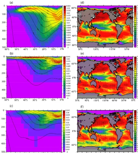
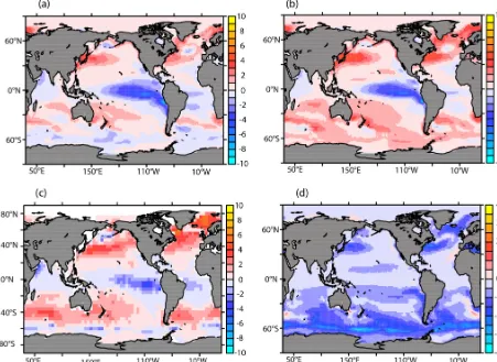
Figure 3. The stratification dρ0/dz(colors) is shown, averaged over the central South Pacific (160◦E–100◦W), for (a) the ARGO-extended data product of de Boyer Montégut et al. (2004), (b) CNTRL, and (c) WSTIR. For each case, potential density contours are overlaid. Also shown is the amplitude of the seasonal cycle of sea surface temperature (SST) (◦C) from (d) the product of Reynolds and Smith (1994) including remote sensing data, (e) for the climatology of the CNTRL run over 2000–2006, and (f) for the climatology of the WSTIR run considered over 2000–2006.
that the1σ0=0.03 corresponds to what was originally pub-lished by de Boyer Montegut et al. (2004). There are large differences not only in summer, where the contrast is be-tween 50 m (1σ0=0.01) and 65 m (1σ0=0.03), but also in winter, where the contrast is between 150 m (1σ0=0.01)
and 200 m (1σ0=0.03). This sensitivity is consistent with what was shown by Holte and Talley (2009).
from the Argo-derived climatology of Roemmich and Gilson (2009). The Argo-derived data product (Fig. 3a) reveals a relatively weak stratification over the Southern Ocean. The stratification is significantly stronger than the observations for the CNTRL case (Fig. 3b) over the Southern Ocean, but relatively weak for the WSTIR case (Fig. 3c). The stratifi-cation maximum is shallower for WSTIR than it is for ob-servations over the Southern Ocean, but is shallower still for CNTRL.
We consider next the amplitude of the seasonal cycle of sea surface temperature (SST), considered for a climatol-ogy constructed for years 2000–2006. This is considered first in Fig. 3d for the observational product derived using the method of Reynolds and Smith (1994), which includes re-mote sensing information. Over large parts of the Southern Ocean, the amplitude of the seasonal cycle of SST is on the order of 2◦C. The distribution shown for the CNTRL run in
Fig. 3e exhibits seasonal variability over the Southern Ocean that is much too large. For the WSTIR run shown in Fig. 3f, it can be seen that the seasonal amplitude of SST is much smaller than for CNTRL, with variations on the order of 2◦C seen over much of the Southern Ocean. The seasonal ampli-tude of SST in the WSTIR run is slightly smaller than that in the observational product in Fig. 3d, but it is generally in better agreement with the observational product than the CNTRL run. These large differences between WSTIR and CNTRL exist despite the fact that both runs have an effective relaxation of SST to the same air temperature field in the bulk formulas used for gas exchange. The tendency of SST in CN-TRL to be too warm in summer is consistent with the over-stratification seen in Fig. 3b, as well as a self-reinforcing diminished heat capacity associated with the strong shallow bias in summertime mixed layer depth seen in Fig. 2b. Inter-estingly, the amplitude of the seasonal cycle of heat content (not shown) is larger for the WSTIR case than for the CN-TRL case over the Southern Ocean, in contrast to what is found for SST.
3.2 Influence of enhanced wind stirring on carbon uptake
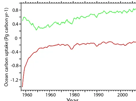
We next consider the decadal-timescale differences in the air–sea exchange of carbon for the two model runs. South-ern Ocean carbon uptake (integrated over the region south of 45◦S) is greater for CNTRL than for WSTIR (Fig. 4), with this difference increasing over time. In the discus-sion here, we ignore the original 5-year adjustment pe-riod for the original shock starting in 1958. This offset and the different evolution of these two simulations have pro-found implications for the role of the Southern Ocean in the global carbon cycle. The WSTIR run results in car-bon outgassing over the Southern Ocean while the CNTRL run simulates carbon uptake throughout the 1965–2006 pe-riod. The outgassing in WSTIR decreases slightly at a rate of 0.05 Pg C yr−1decade−1over the period 1965–2006. For
0.8 0.4
0
-0.4 -0.8
-1.2
1960 1960 1980 1990 2000
O
cean car
bon uptake (P
g car
bon yr
-1)
[image:8.612.315.540.66.233.2]Year
Figure 4. Interannually varying simulated CO2fluxes over 1958– 2006 as a 12-month running mean, with WSTIR in red and CNTRL in green; (units of Pg C yr−1).
CNTRL, carbon uptake increases over the 40-year interval at a rate of 0.125 Pg C yr−1decade−1. The simulated South-ern Ocean fluxes between the CNTRL and WSTIR runs thus diverge at a rate of 0.075 Pg C yr−1decade−1between 1965 and 2006. The difference in uptake between CNTRL and WSTIR is on the order of 0.9 Pg C yr−1at the end of the sim-ulation (averaged over 2000–2006). The difference between these two runs, which represents uncertainty associated with physical mixing and our ability to model it, is very large when compared to the magnitude of inferred perturbations reported elsewhere for the Southern Ocean uptake of con-temporary carbon in response to increasing westerly winds (Le Quéré et al., 2007; Lovenduski et al., 2008; Zickfeld et al., 2007).
Figure 5. Air–sea CO2fluxes for WSTIR averaged over 2000–2006 (a), Air–sea CO2fluxes for CNTRL averaged over 2000–2006(b), Air–sea CO2fluxes for the climatology of Takahashi et al. (2009) focused on the year 2000 (c), and the air–sea flux differences between the WSTIR and CNTRL simulations (d). In all panels, the units are moles C m−2yr−1. Positive values indicate carbon uptake by the ocean.
3.3 Wind stirring and the seasonal cycles of biogeochemical fields
Lenton et al. (2013) demonstrated in their Southern Ocean synthesis study that ocean carbon models contain significant biases in their representation of the seasonal cycle of air– sea CO2fluxes over the Southern Ocean. One of their main conclusions was that identifying uncertainties related to spe-cific processes operating over the seasonal cycle should be a priority for future Southern Ocean carbon cycle research. Given that the seasonal timing of re-stratification and de-stratification, as well as mean summer mixed-layer depths, exercise a fundamental control on upper ocean biogeochem-istry, we are motivated to consider here the effect of the wind-stirring parameterization on the climatological seasonal cycle of various biogeochemical variables. To this end, we char-acterize the sensitivity of the biogeochemical fields to the perturbations imposed on the physical state as considered in Figs. 2 and 3.
3.3.1 Carbon and oxygen fluxes
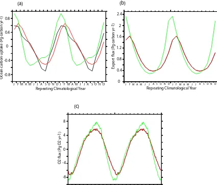
The climatological seasonal cycle of air–sea CO2 flux, in-tegrated south of 45◦S, is shown in Fig. 6a for CNTRL, WSTIR, and for the data product derived from Takahashi et al. (2009). Observations show that ocean CO2uptake, rela-tive to the annual mean, occurs in austral summer and out-gassing occurs during austral winter. There are significant differences in phase, magnitude, and shape between CNTRL and WSTIR. It is nevertheless clear that this sensitivity is less than the CMIP5 model spread in evidence in Fig. 15b of Anav et al. (2013). Independent sensitivity studies with the PISCES model with the parameter setting in the Geider et al. (1998) representation of growth rates (not shown) in-dicate a sensitivity that is even larger than that found with mixed-layer depth. Thus, differences in model representation of wind stirring are only expected to contribute part of the difference illustrated by Anav et al. (2013).
(c)
(a) (b)
2.4
1.6 2
1.2
0.8
0.4
0 J F M A M J J A S O N D J F M A M J J A S O N D Repeating Climatological Year
Expor
t flux (P
g car
bon yr
-1)
J F M A M J J A S O N D
0 4 8
-4
-8
J F M A M J J A S O N D
Repeating Climatological Year
O2 flux (P
g O2 yr
-1)
-0.4
-0.8
J F M A M J J A S O N D J F M A M J J A S O N D Repeating Climatological Year
0.4 0.8
0
O
cean car
bon uptake (P
g car
bon yr
[image:10.612.91.510.66.242.2]-1)
Figure 6. Time variability of Southern Ocean (45–90◦S) fluxes in units of petagrams per year: (a) climatological seasonal cycle of air–sea CO2fluxes, for the climatology of Takahashi et al. (2009) using the gas exchange parameterization of Wanninkhof (1992) in black, the WSTIR case in red, and the CNTRL case in green; (b) climatological seasonal cycle of carbon export over the Southern Ocean, showing WSTIR (red) and CNTRL (green); (c) climatological seasonal cycle of air–sea O2fluxes, for WSTIR (red) and CNTRL (green).
production and enhances the biological drawdown of dis-solved inorganic carbon (DIC) in the ocean’s surface layer earlier in the season for CNTRL than for WSTIR. Inclusion of the ad hoc wind stirring parameterization delays the onset of the winter reversal from outgassing to ingassing by 3 to 4 months (Fig. 6a) relative to CNTRL. The winter outgassing peak in CNTRL, however, is much too early relative to observations.
Aside from changing the phasing and amplitude of the seasonal cycle, the ad hoc parameterization also impacts the skewness of the climatological seasonal cycle of air–sea CO2 fluxes. The exaggerated skewness found for CNTRL relative to the observational product and WSTIR at least in part re-flects the sharp skewness in biological processes revealed in the diagnostic of seasonality in export (Fig. 6b). The sharp peak in export production in January for CNTRL relative to WSTIR is a consequence of light limitation being less for
CNTRL relative to WSTIR. Integrated over the seasonal cy-cle, the Southern Ocean export is 1.48 Pg C yr−1for WSTIR and 2.33 Pg C yr−1for CNTRL. Southern Ocean carbon ex-port in CNTRL is thus 58 % larger than in WSTIR even if, globally, both have nearly identical annual mean export val-ues of 7.4 Pg C yr−1.
[image:10.612.87.512.67.429.2]O2flux cycle is approximately 25 % larger for CNTRL than for WSTIR.
Clearly the sensitivity of O2 fluxes to the ad hoc wind stirring parameterization does not perfectly mirror the sen-sitivity seen for CO2 fluxes in Fig. 6a. Differences in the impact on the seasonality of O2and CO2 fluxes should be expected, given that air–sea equilibration timescales for O2 are approximately an order of magnitude more rapid than for CO2. However, differences in entrainment of O2 and CO2 across the base of the mixed layer are also expected to be important.
Given the relatively short duration of the WSTIR pertur-bation relative to CNTRL (decades), it should be emphasized that this sensitivity of air–sea fluxes of contemporary carbon does not provide insight into the future 21st century uptake capacity of the Southern Ocean to anthropogenic carbon. The analysis also reveals that the differences are manifested in O2 fluxes, with the perturbations to O2 not being perfectly redundant to the changes in CO2fluxes.
3.3.2 Chlorophyll and blooms
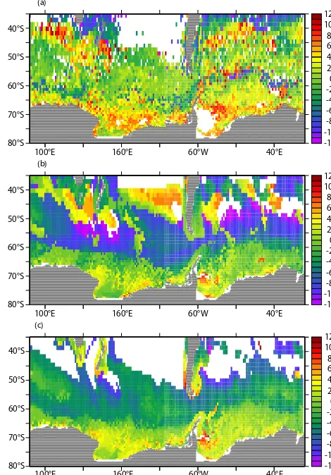
Remotely sensed surface chlorophyll from the Sea-viewing Wide Field-of-view Sensor (SeaWiFS, http://oceancolor. gsfc.nasa.gov/) is used here as a metric to evaluate the mod-eled seasonal cycle and ecological effects of the wind stirring parameterization. A seasonal climatology was constructed over the period 1998–2006 to address both the timing of maximum seasonal chlorophyll concentrations and the tim-ing of bloom onset. To create the climatology, SeaWiFS data were first put on the same grid as the ocean model. Modeled chlorophyll and regridded SeaWiFS data were then averaged to 8-day mean fields. In order to focus on local comparisons and minimize extrapolation errors due to missing data where storms and other phenomena have obscured data retrieval, the model was sampled only at space-time coordinates where SeaWiFS observations are available.
The timing of the climatological maximum chlorophyll concentrations is considered in Fig. 7 for SeaWiFS (Fig. 7a), CNTRL (Fig. 7b), and WSTIR (Fig. 7c). The timing of max-imum chlorophyll concentrations has better agreement with observations for WSTIR than for CNTRL. Within the lat-itude band 50–60◦S, the SeaWiFS product indicates peak concentrations largely within November and December, with early November maxima tending to fall along 60◦S. For CN-TRL, there are large expanses where September maxima are in evidence over 50–60◦S, thereby leading the observations
in phase by as much as 2 months. For the WSTIR case, the phase lead is on the order of 1 month relative to the observa-tions.
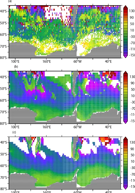
We then consider the timing of bloom onset shown in Fig. 8. The onset timing was chosen for each surface grid point as the time when chlorophyll concentrations increased above the median level plus 0.2 mg m−3during the 4-month period preceding the seasonal chlorophyll maximum (a
for-40°S
50°S
60°S
70°S
80°S
100°E 160°E 60°W 40°E -120 -100 -80 -60 -40 -200 20 40 60 80 100 120
40°S
50°S
60°S
70°S
80°S
100°E 160°E 60°W 40°E -120 -100-80 -60 -40 -200 20 40 60 80 100 120
40°S
50°S
60°S
70°S
80°S
100°E 160°E 60°W 40°E -120 -100-80 -60 -40 -200 20 40 60 80 100 120 (a)
(b)
[image:11.612.310.545.69.406.2](c)
Figure 7. Seasonal phasing of the peak chlorophyll concentrations
for (a) SEAWIFS, (b) CNTRL, and (c) WSTIR; units are days for a climatological year. Regions where the quantity is not well or de-fined or where the quantity and/or bloom are not well-dede-fined are shown in white.
mulation considering the median plus 5 % was also tried, but this multiplicative formulation had trouble in cases with a double-peak seasonal cycle of chlorophyll). Bloom onset is shown for SeaWiFS (Fig. 8a), CNTRL (Fig. 8b), and WSTIR (Fig. 8c).
40°S
50°S
60°S
70°S
80°S
100°E 160°E 60°W 40°E
90 130
40°S
50°S
60°S
70°S
80°S
100°E 160°E 60°W 40°E
40°S
50°S
60°S
70°S
80°S
100°E 160°E 60°W 40°E
50 10 -30 -70 -110 -150
90 130
50 10 -30 -70 -110 -150
90 130
50 10 -30 -70 -110 -150
(a)
(b)
[image:12.612.51.285.69.403.2](c)
Figure 8. Phasing of the bloom onset timing for (a) SEAWIFS, (b)
CNTRL, and (c) WSTIR; units are days for a climatological year. Regions where the quantity is not well or defined or where the quan-tity and/or bloom are not well-defined are shown in white.
3.4 Influence of increased wind stirring on atmospheric potential oxygen
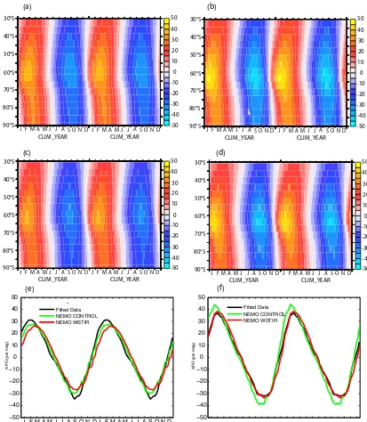
Next we consider the simulations of atmospheric potential oxygen (APO) for the two models. The observed and sim-ulated climatological seasonal cycles of APO at Cape Grim (CGO) station in Tasmania (40.68◦S, 144.69◦E) and Palmer Station (PSA) station on the Antarctic Peninsula (64.46◦S, 64.03◦W), two stations from the Scripps network, are shown in Fig. 9. Cape Grim (Fig. 9e) is located north of the Antarc-tic Circumpolar Current (ACC) and is thereby a footprint region that is subtropically influenced, in contrast to PSA (Fig. 9f), which is located south of the ACC.
For the models the climatological seasonal cycle is cal-culated using daily output, and for the observations weekly flask measurements (snapshots) are used. As a first step, the model output and the data are interpolated onto a regular weekly time grid using a seasonal-trend decomposition by loess (STL) algorithm (Cleveland et al., 1990), which cal-culates a gradually evolving seasonal cycle and trend for
time series data without including any assumptions about the functional form of these quantities. The data is then de-trended by subtracting the seasonal cycle that is calculated using STL, and a climatological mean seasonal cycle is cal-culated. Hovmöller diagrams showing the seasonal cycle of APO as a function of latitude for WSTIR and CNTRL are shown in Fig. 9a and b. In both cases, the APO has been detrended to emphasize the phasing and amplitude of the cli-matological seasonal cycle of each latitude band.
The seasonal maximum APO occurs later for WSTIR (Fig. 9a) than for CNTRL (Fig. 9b), and the amplitude of the seasonal cycle over the latitude range 60–65◦S is larger for CNTRL than for WSTIR. Additionally, the WSTIR max-imum (January to March) peak is broader than the CNTRL peak. These differences in phase and amplitude are domi-nated by O2 (relative to CO2 and N2, not shown) and are consistent with the phase shift in O2fluxes over the Southern Ocean between the CNTRL and WSTIR cases (Fig. 6c). In order to test the importance of the O2contribution to the to-tal APO signal, the variations driven by the O2fluxes alone, with the N2 and CO2components held at a constant value, are considered explicitly for WSTIR (Fig. 9c) and CNTRL (Fig. 9d). These two panels reveal the dominance of surface O2fluxes in driving the total APO signal over the extratrop-ics of the Southern Hemisphere when compared to the fields shown in Fig. 9a and b. The O2contribution alone is consid-ered explicitly for WSTIR (Fig. 9c) and CNTRL (Fig. 9d), revealing the dominance of this contribution to the total APO signal.
The observed climatological seasonal cycles of APO from site CGO and PSA are shown in Fig. 9e and 9f, where they are also compared with the seasonal cycle from CNTRL and WSTIR. At CGO, the simulated APO seasonal cycle is in good agreement between CNTRL and WSTIR (Fig. 9e), al-though the seasonal amplitude for both CNTRL and WSTIR is slightly smaller than observed. The wind stirring perturba-tion has only a minor effect on the seasonal cycle of APO north the ACC, in agreement with Fig. 9b.
At PSA (Fig. 9f), which is south of the ACC, the seasonal cycle of CNTRL has a distinctively greater magnitude and is slightly phase shifted, leading slightly the seasonal cycle of WSTIR. The phasing of the seasonal cycle for WSTIR is in better agreement with the observations at PSA than for CN-TRL. However, from this analysis alone it is not yet clear how the relative contributions of atmospheric O2and CO2 varia-tions contribute to the phasing of APO at PSA for WSTIR and CNTRL (Fig. 9f). The sensitivity of APO to the wind stirring parameterization is stronger south of the ACC be-cause the near surface oceanic vertical O2concentration gra-dient is larger to the south of the ACC than to the north of it.
−50 −40 −30 −20 −10 0 10 20 30 40 50
APO (per meg)
J F M A M J J A S O N D J F M A M J J A S O N D
Fitted Data NEMO CONTROL NEMO WSTIR (b) (a) 30°S 60°S 50°S 40°S 70°S 80°S 90°S -50 -40 -30 -20 -10 0 10 20 30 40 50
J F M A M J J A S O N D J F M A M J J A S O N D
CLIM_YEAR CLIM_YEAR 30°S 60°S 50°S 40°S 70°S 80°S 90°S -50 -40 -30 -20 -10 0 10 20 30 40 50
J F M A M J J A S O N D J F M A M J J A S O N D
CLIM_YEAR CLIM_YEAR 30°S 60°S 50°S 40°S 70°S 80°S 90°S -50 -40 -30 -20 -10 0 10 20 30 40 50
J F M A M J J A S O N D J F M A M J J A S O N D
CLIM_YEAR CLIM_YEAR 30°S 60°S 50°S 40°S 70°S 80°S 90°S -50 -40 -30 -20 -10 0 10 20 30 40 50
J F M A M J J A S O N D J F M A M J J A S O N D
CLIM_YEAR CLIM_YEAR −50 −40 −30 −20 −10 0 10 20 30 40 50
J F M A M J J A S O N D J F M A M J J A S O N D
APO (per meg)
Fitted Data NEMO CONTROL NEMO WSTIR
(c) (d)
[image:13.612.92.505.65.539.2](e) (f)
Figure 9. Atmospheric potential oxygen (APO) as simulated by the atmospheric transport model (ATM), in per meg units, for a detrendended
climatological cycle. In each panel, the seasonal cycle is represented twice. Hovmöller diagram of canonical seasonal cycle of zonal mean surface APO for CNTRL case (a); Hovmöller diagram of canonical seasonal cycle of zonal mean surface APO for WSTIR case (b); Hov-möller diagram showing the relative contribution of O2to climatological APO variations for WSTIR (c); Hovmöller diagram showing the relative contribution of O2to climatological APO variations for CNTRL (d); Cape Grim, Australia (CGO): Repeated climatological seasonal cycle compared with observations from Scripps network; here the climatological seasonal cycle is calculated using the STL analysis tools of Cleveland et al. (1990) (e). Palmer Station, Antarctica (PSA): Repeated climatological seasonal cycle compared with observations from Scripps network; Here the climatological seasonal cycle is calculated using the STL analysis tools of Cleveland et al. (1990) (f).
APO over years 1998 to 2011. For each realization of the sea-sonal cycle, we consider the time interval 1 July to 30 June as a separate line over years 1998 to 2011. For each case, the seasonal cycle is repeated twice with the same line to fa-cilitate interpretation. For the decade that corresponds to the
J F M A M J J A S O N D J F M A M J J A S O N D −50
−40 −30 −20 −100 10 20 30 40 50
APO (per meg)
J F M A M J J A S O N D J F M A M J J A S O N D −50
−40 −30 −20 −100 10 20 30 40 50
APO (per meg)
J F M A M J J A S O N D J F M A M J J A S O N D −50
−40 −30 −20 −100 10 20 30 40 50
APO (per meg)
J F M A M J J A S O N D J F M A M J J A S O N D −15
−10 −5 0 5 10 15
APO (per meg)
J F M A M J J A S O N D J F M A M J J A S O N −15
−10 −5 0 5 10 15
APO (per meg)
J F M A M J J A S O N D J F M A M J J A S O N D −15
−10 −5 0 5 10 15
APO (per meg)
(a)
(b)
(c)
(d)
(e)
[image:14.612.69.525.71.425.2](f)
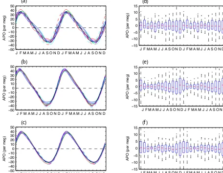
Figure 10. Atmospheric potential oxygen (APO), with each year shown separately over 1 July–30 June. (a) Observations from Scripps
network, with each line corresponding to a separate year but repeated twice to facilitate interpretation. Each line represents a different year between 1998 and 2011. Solid lines are used for years that overlap with the model runs (1998–2005), while dashed lines are used for the more recent observations. (b) Model output from the CNTRL case over the period 1994–2005, with each line corresponding to a separate year but repeated twice. Solid lines are used for years that overlap with the observations (1998–2005), while dashed lines are used for the earlier period. (c) Model output from the WSTIR case, with each line corresponding to a separate year but repeated twice. Time period follows
(b). (d) Observations, bar and whiskers plot of intraseasonal variability inferred from STL analysis, with red lines showing mean (per meg)
deviations, and blue boxes marking 25th and 75th percentile values of intraseasonal variations. Bars represent the full range of values, but outliers defined as values larger than 1.5 times the interquartile range, have been excluded. Time period follows (a). (e) Same as (d), but for CNTRL. Time period follows (b). (f) Same as (e), but for WSTIR. Time period follows (b).
and the phase of the seasonal periods of increasing and de-creasing APO. We infer from what we have seen in Fig. 9f for Palmer Station climatologies that APO is sensitive to the phasing of the re-stratification and de-stratification over the Southern Ocean. Might this inference from a comparison of the respective WSTIR and CNTRL climatologies be sup-ported by either of the runs considered individually?
Clearly for the individual cases of WSTIR (Fig. 10b) and CNTRL (Fig. 10c) considered separately, the year-to-year variations in the phase and amplitude of the seasonal cycle are significantly smaller than what is seen in the observations (Fig. 10a). This is an important illustration of both the power
Next we consider intraseasonal variations in APO as in-ferred for Palmer Station for both the observations and the two model runs in bar and whiskers diagrams. A second-order low-pass Butterworth filter was applied to weekly mean observations and model output fields with a cutoff fre-quency of 1/6, retaining information with frequencies lower than 6 weeks. The panel for Palmer Station (Fig. 10d) re-veals the median (red line), the 25th–27th percentile varia-tions (black box). Outliers, which are defined as being more than 1.5 times the inter-quartile variations, are not shown. The whiskers show the highest and lowest excursions that are not considered outliers for each month. Importantly, the in-traseasonal variations reveal amplitude modulations over the seasonal cycle, with variations in austral spring (on the order of 15 per meg) twice as large as variations in austral autumn. From this analysis alone, it is not clear whether intraseasonal processes in the ocean or the atmosphere (or both) drive the intraseasonal variations in APO with inherent timescales on the order of weeks.
The intraseasonal variations for the CNTRL run (Fig. 10e) and the WSTIR run (Fig. 10f) are qualitatively similar to the observations in terms of modulations of the amplitude over the seasonal cycle. Nevertheless there are important differ-ences between CNTRL and WSTIR. The timing of maxi-mum amplitude intraseasonal variations in CNTRL during austral spring peaks earlier than in WSTIR, even though the atmospheric transports used for these two APO simulations are identical. This implicates the surface air–sea fluxes driv-ing APO variations as bedriv-ing important. It is still not clear if this occurs through their slowly varying impact on the mean meridional gradients in APO during spring or through in-traseasonal variations in the surface fluxes themselves, since the atmospheric simulations were forced with daily varying air–sea fluxes. As can be seen in Fig. 9a and b, large-scale meridional gradients in APO at the latitude of Palmer Station are not pronounced in either WSTIR or CNTRL in austral spring, and are thereby the variations in evidence in Fig. 10d are consistent with elevated intraseasonal variability in air– sea fluxes in austral spring.
Within the larger context of climatologies emphasized in this paper, we wish to emphasize that the APO measured at Palmer Station exhibits information over a broad range of timescales. It is not yet clear whether the year-to-year changes in the phasing of the seasonal cycle (Fig. 10a) are independent of the modulations of intraseasonal variability (Fig. 10b). Nevertheless the intraseasonal variations in APO are not randomly distributed over the seasonal cycle.
3.5 Influence of wind stirring on surface and interior nutrient distributions
We also consider the impact of wind stirring on surface nutrients Fe and NO3. The concentration of Fe averaged over 2000–2006 is shown for WSTIR (Fig. 11a), CN-TRL (Fig. 11b), and the difference between these two runs (Fig. 11c). Likewise, the analogous distributions for NO3are shown for WSTIR (Fig. 11d), CNTRL (Fig. 11e), and the difference (Fig. 11f).
This reveals that the annual mean Fe concentrations are lower for WSTIR than for CNTRL, while the annual mean NO3 concentrations are higher. Enhanced summer entrain-ment for WSTIR relative to CNTRL should sustain both higher Fe and NO3 concentrations, but under light-limited conditions, Fe and NO3have different response functions, re-sulting in a situation where NO3increases but Fe decreases when vertical mixing increases. For NO3, enhanced light limitation associated with enhanced mixed-layer depths re-sults in high surface NO3concentrations relative to CNTRL, adding to the entrainment signal. For Fe, on the other hand, the Fe/DIC ratio of biological uptake increases as a con-sequence of light limitation, and biology consumes increas-ingly more Fe, thereby driving a tendency towards decreased Fe concentrations. This behavior is common to biogeochem-ical models over the Southern Ocean by design, but Strzepek et al. (2012) have recently argued that this is not consistent with observations. This strong sensitivity demonstrated here, and the controversy surrounding it, should serve to motivate further work to understand how the Fe/DIC ratio changes under light limitation.
What are the consequences for NO3and DIC distributions in the ocean interior? In Fig. 12, we consider the distribution of NO3 and DIC concentrations projected onto σ0=26.8 (Subantarctic Mode Water (SAMW) density class), with av-eraged concentrations calculated over the period 2000–2006. The two runs were “split” in 1958, and thus this represents a perturbation signal of approximately 45 years. The distri-bution of NO3is shown for WSTIR (Fig. 12a), for CNTRL (Fig. 12b), and for the difference between these two runs (Fig. 12c). The interior concentration of NO3 is higher for WSTIR than for CNTRL, consistent with Fig. 11f consid-ering the outcrop latitude of theσ0=26.8 isopycnal. Given that the difference in NO3concentrations reflects the signal ∼45 years into the perturbation, it is not surprising that the perturbation is largest over the Southern Hemisphere sub-tropical gyres given the multi-decadal timescales for this re-gion (see Fig. 3 of Rodgers et al. (2003) for relevant La-grangian diagnostics), with a smaller-amplitude signal hav-ing accessed via ocean interior transport the equatorial up-welling region of the Pacific.
Figure 11. Surface concentrations are shown averaged over years 2000–2006 for (a) Fe in WSTIR, (b) Fe in CNTRL, and (c) the difference
in Fe between WSTIR and CNTRL (units of nM). Surface concentrations are shown averaged over years 2000–2006 for (d) NO3in WSTIR,
(e) NO3in CNTRL, and (f) the difference in NO3between WSTIR and CNTRL (units of µM).
biological productivity is fueled by nutrients exported from the Southern Ocean in the SAMW density class. Viewed as an estimate of uncertainty, the results presented here for NO3 concentrations underscore the potential importance of wind stirring over the Southern Ocean for larger-scale nutrient sup-ply over the global ocean.
In Fig 12d and e we consider the simulated DIC concen-trations for both model WSTIR and CNTRL for the same
Figure 12. Ocean interior concentrations (σ0=26.8) are shown averaged over years 2000–2006 for (a) NO3in WSTIR, (b) NO3in CNTRL, and (c) the difference in NO3between WSTIR and CNTRL (units of µM). Ocean interior concentrations (σ0=26.8) are shown averaged over years 2000–2006 for (d) DIC in WSTIR, (e) DIC in CNTRL, and (f) the difference in DIC between WSTIR and CNTRL (units of µM).
for the NO3distributions considered in the same figure. How-ever, the perturbation structure in DIC is markedly different from that seen in NO3. First, the DIC perturbations are as large in the Northern Hemisphere as they are in the Southern Hemisphere for DIC, whereas this is not the case for NO3. Second, for NO3 the perturbations suggest advective prop-agation, with maxima moving inward from SAMW
NO3. The complex interplay between these processes, and their impact on the transport of DIC and NO3 northwards from the Southern Ocean, is left as a subject for future inves-tigation.
4 Discussion
The sensitivity of contemporary CO2 uptake to a change in wind stirring is significantly larger than the previously reported sensitivity to local wind speed perturbations and gas exchange formulations that impact piston velocity alone (Sarmiento et al., 1992). This is important given the multi-faceted role of winds in impacting exchanges of properties across the air–sea interface, as tabulated in the Introduction, and suggests the need to generalize the conceptual model of gas exchange beyond the framework of piston velocities. In fact, not only is the sensitivity found here significantly stronger, but it is also of opposite sign to what is found for surface gas exchange parameterizations, with enhanced wind stirring driving the reduced uptake of contemporary carbon over the Southern Ocean (Fig. 5).
The model revealed a large sensitivity in contemporary carbon uptake over the Southern Ocean not only for a cli-matological seasonal cycle (seasonal deviations from the an-nual mean), but also over interanan-nual and longer timescales (Fig. 4). For the seasonal cycle, the CNTRL case exhibits a shift in phase towards earlier spring CO2 uptake relative to WSTIR. This is a consequence of the combined impacts of biology (through light limitation) of the earlier stratification for CNTRL relative to WSTIR, as evidenced in the earlier manifestation of the Chl concentration maximum for CN-TRL relative to WSTIR (Fig. 7), and the reduced physical entrainment for CNTRL of higher-DIC waters from below.
The sensitivity of Southern Ocean carbon cycling and bio-geochemistry to wind stirring should also be expected to have implications for model-derived estimates of the time-evolution of carbon uptake. Interpreting the 0.9 Pg C yr−1 difference in integrated air–sea uptake of CO2over the re-gion to the south of 45◦S between CNTRL and WSTIR over 2000–2006 as an uncertainty associated with our imper-fect knowledge of how to represent wind stirring in models, it is important to consider this uncertainty within the con-text of the debate waging in the carbon cycle community over whether an ocean carbon-climate feedback is already in evidence in air–sea CO2 fluxes. In fact, this uncertainty identified here is at least of the same order as the global carbon-climate feedback presented in the study of Le Quéré et al. (2007) of 0.2±0.2 Pg C yr−1, and the same holds for results presented by Zickfeld et al. (2007) and Lovenduski et al. (2008).
The question arises as to whether the time interval over which we considered the sensitivity to wind stirring (1958– 2006) is of sufficient duration to distinguish between spu-rious signals associated with adjustments, trends that
repre-sent the real response of the system to perturbations, and the longer-term steady-state response of the system. The rela-tively short duration (several years) of the spurious adjust-ment signal in Fig. 4 reveals that our interests in both the adjustment period and the long-term steady-state response of the system can be met. The adjustment over decadal timescales is directly pertinent to the type of decadal secular trend in the strength of reanalysis winds over the Southern Ocean as reported by Le Quéré et al. (2007). Such increases in the wind strength (considered in the annual mean and in-tegrated over the Southern Ocean) should be expected to be directly connected to an increase in storminess. Such an in-crease in the input of high-frequency (less than 10-day) en-ergy from the winds may be expected to contribute to destrat-ifying the planetary boundary layer of the ocean through an increased input of potential energy. This also serves as confir-mation of our central hypothesis, namely that by perturbing the transfer of energy from the atmosphere to the ocean, both the steady state and the variability/trends are perturbed.
The strong sensitivity of winter mixed-layer depths to wind stirring (reflected in the green and red lines in Fig. 2d) warrants comment as well. This is scientifically interesting, as it is related to the mechanical forcing provided by the winds and not to heat fluxes or other processes that change sign with the march of the seasons. The deeper mixing in winter for WSTIR relative to CNTRL largely reflects pre-conditioning or erosion of the stratification below the base of the mixed layer that occurs during summer, with only mini-mal erosion of stratification occurring through wind stirring in winter given the limited depth scale over which the param-eterization is applied. This serves to complement our earlier comments on the impact of wind stirring on the phase of the seasonal cycle of mixed-layer depth. This may help to provide insight not only into mechanisms, but also into the CMIP5 modeled mixed-layer depth biases of the type con-sidered by Sallée et al. (2013).
experiment. The critical point to learn from the results pre-sented here is that the representation of vertical mixing in the model caused important changes in the biogeochemical state from the equilibrium state, demonstrating that our un-derstanding of the dynamical controls on ocean biogeochem-istry remains limited.
5 Conclusions
The main goal of this study was to investigate the sensitivity of CO2 uptake over the Southern Ocean and, more gener-ally, Southern Ocean biogeochemistry, to an ad hoc parame-terization of wind stirring. The ad hoc wind stirring param-eterization was developed to account for processes associ-ated with shear-induced turbulence that are commonly unac-counted for in ocean models, whereby summer mixed-layer depths tend to be too shallow over the Southern Ocean and in particular under the maximum westerlies. The ad hoc pa-rameterization, which by construction acts with an e-folding scale depth of 60 m over the Southern Ocean, was used to tune the NEMO mixed-layer depths to better resemble Argo-derived distributions.
The wind stirring parameterization impacts not only the penetration depth of austral summer (DJF) mixed layers, but also the seasonal cycle and phasing of stratification and de-stratification over the Southern Ocean, particularly in the region of maximum westerlies. With the parameterization, mixed layers remain deeper than 60 m for 5 weeks longer than without the parameterization in the region between 50◦S and 60◦S. This has important implications for
South-ern Ocean carbon cycling, vertical carbon export, SouthSouth-ern Ocean biogeochemistry, and for the injection of preformed nutrients in the ocean interior.
In this study we also sought to evaluate the dynamical con-trols exerted by ocean mixing processes on atmospheric po-tential oxygen (APO). Our main scientific finding was that wind stirring exerts a strong control on the phasing of the seasonal cycle of APO, primarily through its impact on the seasonality of air–sea O2 fluxes, with the sensitivity being stronger to the south of the ACC than to the north of the ACC. In the observations we also identified significant year-to-year and intraseasonal variations in the seasonality of APO for Palmer Station. These variations in APO on timescales sig-nificantly shorter than the seasonal cycle should be explored mechanistically in a further study. The intraseasonal varia-tions may reflect the response timescales of APO to synoptic-scale storms, but it is not yet clear to what degree they reflect oceanic and/or atmospheric processes. Give that storminess is expected to increase under 21st century climate change (Wu et al., 2010), it will be important in future work to iden-tify whether they impact ocean biogeochemistry over large scales.
Increasing wind stirring by including the ad hoc param-eterization reduces Southern Ocean (<45◦S) carbon
up-take by 0.9 Pg C yr−1 over years 2000–2006 relative to the overly stratified control simulation. Wind stirring not only increases summertime mixed-layer depths, thereby impact-ing light limitation and entrainment of nutrients from below, but it also impacts the phasing of the seasonal cycle and, more generally, biogeochemistry by delaying the timing of re-stratification in spring. Over the Southern Ocean, wind stirring also decreases export production by 0.85 Pg C yr−1, nearly the same amount by which it reduced ocean uptake of CO2by gas exchange.
Although inclusion of the ad hoc wind stirring param-eterization leads to improvements in the model’s physical oceanic state, globally integrated ocean carbon uptake is only 0.1 Pg C yr−1over 2000–2006 with the ad hoc parameteriza-tion (WSTIR case), much less than the 2.8 Pg C yr−1 sim-ulated without the ad hoc parameterization (CNTRL case) over the same period. This latter value obtained without the effect of enhanced wind stirring is, however, in closer agree-ment with observational estimates of global carbon that are typically between 1.4 and 2.6 Pg C yr−1 for the 1990–2009 period (Wanninkhof et al., 2013). Importantly, this serves as an example of where biogeochemical models can be tuned to simulate global carbon uptake in agreement with observa-tional products even though their physical circulation states are unsatisfactory. This underscores a potentially very large uncertainty in our ability to model future global carbon up-take.
Acknowledgements. The contribution of K. B. Rodgers came through awards NA17RJ2612 and NA08OAR4320752, which includes support through the NOAA Office of Climate Ob-servations (OCO). The statements, findings, conclusions, and recommendations are those of the authors and do not necessarily reflect the views of NOAA or the US Department of Commerce. Additional support for K. B. Rodgers came through NASA award NNX09AI13G and NSF award OCE-1155983. Support for S. E. Mikaloff Fletcher was provided by NIWA under the New Zealand Greenhouse Gas Emissions, Mitigation, and Carbon Cycle Science Programme. Y. Plancherel acknowledges support from the Oxford Martin School and the UK GEOTRACES Program. Support for measurements of APO ratios was provided under grant NA10OAR4320156, which includes support through the NOAA Climate Program Office. D. Iudicone was funded by the Flagship Project RITMARE – The Italian Research for the Sea – funded by the Italian Ministry of Education, University, and Research within the National Research Program 2011–2013. Y. Plancherel was supported by the Oxford Martin School and UK NERC via the UK GEOTRACES program.
Edited by: L. Cotrim da Cunha
References
Anav, A., Friedlingstein, P., Kidston, M., Bopp, L., Ciais, P., Cox, P., Jones, C., Jung, M., Myneni, R., and Zhu, Z.: Evaluating the Land and Ocean Components of the Global Carbon Cycle in the CMIP5 Earth System Models, J. Climate, 6, 6801–6843, 2013. Antonov, J. I., Seldov, D., Boyer, T. P., Locarnini, R. A., Mishonov,
A. V., Garcia, H. E., Baranova, O. K., Zweng, M. M., and John-son, D. R.: World Ocean Atlas 2009, Volume 2: Salinity, in: NOAA Atlas NESDIS 69, edited by: Levitus, S., U.S. Govern-ment Printing Office, Washington DC, 184 pp., 2010.
Aumont, O. and Bopp, L: Globalizing results from ocean in situ iron fertilization studies, Global Biogeochem. Cy., 20, GB2017, doi:10.1029/2005GB002591, 2006.
Axell, L. B.: Wind-driven internal waves and Langmuir circulations in a numerical ocean model of the Southern Baltic Sea, J. Geo-phys. Res., 107, 3204, doi:10.1029/2001JC000922, 2002. Blanke, B. and Delecluse, P.: Variability of the tropical-Atlantic
ocean simulated by a general circulation model with two dif-ferent mixed-layer physics, J. Phys. Oceanogr., 23, 1363–1388, 1993.
Boden, T. A., Marland, G., and Andres, R. J.: Global, Re-gional, and National Fossil-Fuel CO2Emissions, Carbon Diox-ide Information Analysis Center, Oak Ridge National Labo-ratory, U.S. Department of Energy, Oak Ridge, Tenn., USA, doi:10.3334/CDIAC/00001_V2012, 2012.
Bolin, B. and Eriksson, E.: Changes in the carbon dioxide content of the atmosphere and sea due to fossil fuel combustion, in: The Atmosphere and the Sea in Motion: Scientific Contributions to the Rossby Memorial Volume, edited by: Bolin, B., New York, Rockefeller Institute Press, 130–142, 1958.
Böning, C., Dispert, A., Visbeck, M., Rintoul, S., and Scharzkopf, F.: The response of the Antarctic Circumpolar Current to recent climate change, Nat. Geosci., 1, 864–869, 2008.
Brodeau, L., Barnier, B., Treguier, A. M., Penduff, T., and Gulev, S.: An ERA40-based atmospheric forcing for global ocean circulation models, Ocean Model., 31, 88–104, doi:10.1016/j.ocemod.2009.10.005, 2010.
Cleveland, R. B., Cleveland, W. S., McRae, J. E., and Terpenning, I.: STL: A Seasonal-Trend Decomposition Procedure Based on Loess, J. Off. Stat., 6, 3–73, 1990.
de Baar, H. J. W., Boyd, P. W., Coale, K. H., Landry, M. R., Tsuda, A., Assmy, P., Bakker, D. C. E., Bozec, Y., Barber, R. T., Brzezinski, M. A., Buesseler, K. O., Boyé, M., Croot, P. L., Gervais, F., Borbunov, M. Y., Harrison, P. J., Hiscock, W. T., Laan, P., Lancelot, C., Law, C. S., Lavasseur, M., Marchetti, A., Millero, F. J., Nishioka, J., Nojiri, Y., van Oijen, T., Riebe-sell, U., Rijkenberg, M. J. A., Saito, H., Takeda, S., Timmer-mans, K. R., Veldhuis, M. J. W., Waite, A. M., and Wong, C.-S.: Synthesis of iron fertilization experiments: From the Iron Age in the Age of Enlightenment, J. Geophys. Res., 110, C09S16, doi:10.1029/2004JC002601, 2005.
de Boyer Montégut, C., Madec, G., Fischer, A. S., Lazar, A., and Iudicone, D.: Mixed layer depth over the global ocean: An ex-amination of profile data and a profile-based climatology, J. Geo-phys. Res., 109, C12003, doi:10.1029/2004JC002378, 2004. Denning, A. S., Holzer, M., Gurneym, K. R., Heimann, M., Law, R.
M., Rayner, P. J., Fung, I. Y., Fan, S.-M., Taguchi, S., Friedling-stein, P., Balkanski, Y., Taylor, J., Maiss, M., and Levin, I.: Three-dimensional transport and concentration of SF6: A model inter-comparison study (TransCom 2), Tellus B, 51, 266–297, 1999. Dong, S., Sprintall, J., Gille, S. T., and Talley, L.: Southern Ocean
mixed-layer depth from Argo float profiles, J. Geophys. Res., 113, doi:10.1029/2006JC004051, 2008.
Geider, R. J., MacIntyre, H. L., and Kana, T. M.: A dynamic reg-ulatory model of phytoplanktonic acclimation to light, nutrients, and temperature, Limnol. Oceanogr., 43, 679–694, 1998. Gent, P. R. and McWilliams, J. C.: Isopycnal mixing in ocean
cir-culation models, J. Phys. Oceanogr., 20, 150–155, 1990. Gnanadesikan, A.: A simple predictive model for the structure of
the oceanic pycnocline, Sciences, 283, 2077–2079, 1999. Gurney, K. R., Law, R. M., Denning, A. S., Rayner, P. J., Baker, D.,
Bousquet, P., Bruhwiler, L., Chen, Y.-H., Ciais, P., Fan, S., Fung, I. Y., Gloor, M., Heimann, M., Higuchi, K., John, J., Kowal-czyk, E., Maki, T., Maksyutov, S., Peylin, P., Prather, M., Pak, B. C., Sarmiento, J., Taguchi, S., Takahashi, T., and Yuen, C.-W.: TRANSCOM 3 CO2inversion intercomparison: 1. Annual mean control results and sensitivity to transport and prior flux informa-tion, Tellus B., 55, 555–579, 2003.
Hallberg, R. and Gnanadesikan, A.: The role of eddies in deter-mining the structure and response of the wind-driven Southern Hemisphere overturning: Results from the Modeling Eddies in the Southern Ocean (MESO) project, J. Phys. Oceanogr., 36, 2232–2252, 2006.
Hamme, R. C. and Keeling, R. F.: Ocean ventilation as a driver of interannual variability in atmospheric potential oxygen, Tellus B, 60, 706–717, 2008.