Final State Interaction Effects in B
+→J/ψ π
+Decay
H. Mehraban, and A. asadi
*Department of physics, Faculty of sciences, Semnan University P.O.Box 35195-363, Semnan, Islamic Republic of Iran
Received: 4 January 2014/ Revised: 24 February 2014/ Accepted: 15 March 2014
Abstract
In this research the exclusive decay of
is calculated by QCD
factorization (QCDF) method and final state interaction (FSI). First, the
decay is calculated via QCDF method. The result that is found by
using the QCDF method is less than the experimental result. So FSI is considered
to solve the
decay. For this decay,
̅
via the exchange of
mesons are chosen for the intermediate state. The above intermediate
state is calculated by using the QCDF method. In the FSI effects, the results of our
calculations depend on
as the phenomenological parameter. The range of this
parameter is selected from 2 to 3. It is found that if
is selected, the
numbers of the branching ratio are placed in the experimental range. The
experimental branching ratio of
decay is 4.9
and our results
calculated by QCDF and FSI are 0.5
and 3.9
respectively.
Keywords: B meson; QCD factorization; Final state interaction; Intermediate state; Branching ratio.
*
Corresponding author: Tel: + 9353893210; Fax: +231-3354081; Email: [email protected]
Introduction
B meson non-leptonic decays are significant for testing theoretical frameworks and searching new physics beyond the standard model. The next-to-leading order low-energy effective Hamiltonian is used for the weak interaction matrix elements and (FSI). The importance of the FSI in hadronic processes has been identified for a long time. Recently, its applications in D and B decays have attracted extensive interests and attentions of theorists. Since the hadronic matrix elements are fully controlled by non-perturbative QCD, the most important problem is how to evaluate them properly. The factorization method enables one to separate the non-perturbative QCD effects from the
suppressed and the CKM’s most favored two-body intermediate states are the only ones that have been taken into consideration [3]. The FSI can be considered as a soft re-scattering style for certain intermediate
two-body hadronic channel
̅ decay [4]. Therefore, FSI are estimated via the one particle exchange processes at the hadron loop level (HLL) as explained in section 4. We calculated the decay according to QCDF method and BR( ) = 0.5 . The FSI can give sizable corrections. Re-scattering amplitude can be derived by calculating the absorptive part of triangle diagrams. In this decay, intermediate state is ̅ . Then we calculated the
decay according to HLL method. By FSI method we obtain the branching ratio of decay, 3.9 and the experimental result of this decay is 4.9 [5].
We present the calculation of QCDF for decay in Sec. 2. In Sec. 3, we calculate the amplitudes of the intermediate states. Then we present the calculation of HLL for decay in Sec. 4. In Sec. 5, we give the numerical results, and in Sec. 6, we have conclusion.
1. QCD Factorization of Decay
To compare QCDF with FSI, we explore QCDF
analysis. In this section, we obtain the amplitude of decay using QCDF method. In factorization approach, there are color-suppressed tree
and allowed penguin diagrams to
decay. We adopt leading order Wilson coefficients at the scale for QCDF approach. The diagrams describing this decay are shown in Fig.1.
According to the QCDF the amplitude of decay is given by
√ {
[ ]}
Where are the products of elements of the quark mixing matrix. Using the unitarity relation
, we write
∑
And for vector meson , the ratios is defined as
The effective coefficients which are specific to the factorization approach, and defined as
where the quantities of are effective Wilson coefficients at the renormalization scale for the ̅ ̅ transition. In the above amplitude the determination of
in the
current-current transitions has received a lot of attention, the quantities of and are the QCD-penguin and electroweak-penguin coefficients, respectively. Numerical values of ( ) for representative value of the phenomenological parameter
are displayed in Section 5.
2. Amplitudes of Intermediate States
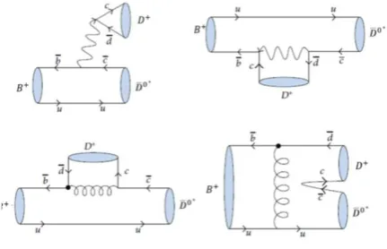
Before analyzing FSI in the decay, we introduce the factorization approach in detail. In FSI effects ̅ is chosen for the intermediate state. For ̅ decay, Feynman diagrams are shown in Fig.2. And the amplitude comes
Figure. 1. The Feynman diagrams contributing to the
decay.
A ( ̅
√ {
√ [
]
(6)
Where are the Wilson coefficients, is the color number and
̅
̅
There are large theoretical uncertainties related to the modeling of power corrections corresponding to weak annihilation effects, we parametrize these effects in terms of the divergent integrals (weak annihilation)
(9)
3. Final State Interaction of Decay
For decay, two-body intermediate state such as ̅ is produced. We can write out the decay amplitude involving HLL contributions with the following formula
Abs M (B(pB) M(p1) M(p2) M(p3) M(p4))
⃗⃗⃗
⃗⃗⃗⃗
for which both intermediate mesons (M1, M2) are
pseudoscalar. And the absorptive part of the HLL diagrams for VP case can be calculated by
Abs M (B(pB) M(p1) M(p2) M(p3) M(p4))
⃗⃗⃗
⃗⃗⃗⃗
{ ( )
}
where ) is the amplitude of that calculated via QCDF method. and involves hadronic vertices factor defined as
⟨ | | ⟩
⟨ | | ⟩
√
⟨ | | ⟩
The dispersive part of the rescattering amplitude can be obtained from the absorptive part via the dispersion relation [6, 7]:
∫
Where is the square of the momentum carried by the exchanged particle and s is the threshold of intermediate states, in this case s . Unlike the absorptive part, the dispersive contribution suffers from the large uncertainties arising from the complicated
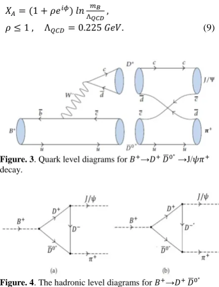
Figure. 3. Quark level diagrams for → ̅ →J/
decay.
integration.
3.1. Final State Interaction In ̅
Decay
The quark model diagram for ̅ decay is shown in Fig.3. And the hadronic level diagrams are shown in Fig. 4.
The amplitude of the mode ̅ are given by
√ ∫
⃗
⃗
( )
⃗⃗⃗ ⃗⃗⃗⃗
| ⃗⃗⃗ || ⃗⃗⃗⃗ | | ⃗⃗⃗ || ⃗⃗⃗⃗ |
⃗⃗⃗⃗ ⃗⃗⃗⃗ , q is the momentum of the exchange is the form factor defined to take care of the off–shell of the exchange particles, which introduced as [8]
The form factor (i.e.n=1) normalized to unity at . and q are the physical parameters of the exchange particle and 𝛬 is phenomenological parameter. It is obvious that for becomes a number. If 𝛬 then turns to be unity, whereas, as the form factor appraochs to zero and the distance becomes small and the hadron interaction is no longer valid. Since 𝛬 shoud not be far from and , we choose
Where the η is the phenomenological parameter that its value in the form factor is expected to be of the order of unity and can be determined from the measured rates, and
√ ∫
⃗
⃗
( √ ) ( √ )
[
]
[ ]
√ ∫ | |
( | | | | || )
(19)
⃗⃗⃗ ⃗⃗⃗⃗
| ⃗⃗⃗ || ⃗⃗⃗⃗ |
| ⃗⃗⃗ || ⃗⃗⃗⃗ |
The dispersion relation is
∫
The decay amplitude of via the HLL diagrams is
4. Numerical Results
Numerical values of effective coefficients for ̅ ̅ transition at are given by [9]
The relevant input parameters used as follows [1, 10, 11]: (The values of the masses and decay constants are in units of GeV)
=1.1 =1.82 (23)
=2.5 1.88 ̅
0.82
1 √
By using the input parameters and according to the
QCDF method of
decay, we get
We note that our estimate of branching ratio of decay according to QCDF method seems less than the experimental result. Before calculating the decay amplitude via FSI, we have to compute the intermediate state amplitude, for the
̅ decay amplitude we get
̅
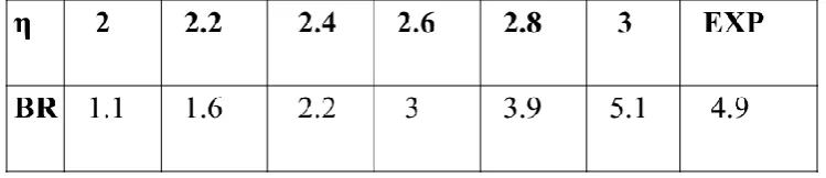
We are able to calculate the branching ratio of decay with different values of η which are shown in Table 1.
Results
In this work, we have calculated the contribution of the t-channel FSI, that is, inelastic re-scattering processes to the branching ratio of decay. For evaluating the FSI effects, we have only considered the absorptive part of the HLL because both hadrons which produced via the weak interaction are on their mass shells. We have calculated the branching ratio of decay by using QCDF and FSI. The experimental result of this decay is BR( )= 4.9 . According to QCDF and FSI, our results are BR( )= 0.5 and 3.9 , respectively.
We have introduced the phenomenological parameter η that its value in the form factor is expected to be of the order of unity and can be determined from the measured rates. For a given exchanged particle, we have used η=2 . If η= 2.8 is selected, the branching ratio of the decay approaches to the experimental bound.
References
1. Cheng H.Y., Chua C. K., Soni A, Final state interactions in hadronic B decay. Phys. Rev D. 71: 014030. 1-59. (2005). 2. Oh Y.S., Song T. and Lee S.H. absorption by and
mesons in a meson exchange model with anomalous parity interactions .Phys. Rev C. 63: 034901. 1-21. (2001). 3. Belyaev V.M., Braun V.M., Khodjamirian A. and Ruchl
R. couplings in QCD. Phys. Rev D. 51:
6177. 1-35. (1995).
4. Mohammadi B. and Mehraban H. Final state interaction in
̅ . J. High Energy Phys. JHEP, 07: 089. 1-11. (2011).
5. Particle Data Group, phys. Rev. D 86: (010001): (2012). 6. Cheng H .Y., Chua C.K., Soni A. Final state interactions in
hadronic B decays . Phys. Rev D. 71(1): 014030. 1-38. (2005).
7. Zhang B., Lu X., Zhu S.L. Dispersive contribution of ρ(1450,1700) decays and X(1576). Chin. Phys. Lett. 24(9): 2537–2539. (2007).
8. Lu C.D. Final state interaction in B → KK decays . Phys. Rev, D. 73(3): 034005. 1-10. (2006).
9. Ali A., Kramer G., Lu C.D. Experimental tests of factorization in charmless nonleptonic twobody B decays .
Phys. Rev D. 58 (9): 094009. 1-40. (1998).
10. Mohammadi B, Mehraban H. final state interactions
effects on the decay. Advances in High Energy Phys. AHEP. 2012: 203692. 1-19. (2012).