Enhanced Calibration of Robot Tool Centre Point
Using Analytical Algorithm
Christof Borrmann
Fraunhofer Institute for Manufacturing Technology and Advanced Materials IFAM, Stade, Germany Email: [email protected]
Jörg Wollnack
Hamburg University of Technology-Institute of Production Management and Technology (IPMT), Hamburg, Germany Email: [email protected]
Abstract—This paper introduces an enhanced method to analytically identify an unknown tool centre point (TCP) of standard industrial robots with six degrees of freedom. The method uses a mathematical closed form to determine the position and orientation (pose) of a mounted robot tool frame in relation to the robot flange frame. This unknown pose is represented by a homogeneous transformation that is calculated by performing two robot movements. The position and orientation of the robot is measured after each movement, which leads to an equation of the form , where represents the unknown homogeneous transformation from the robot flange to the TCP. The achievable accuracy in comparison to existing methods is enhanced by using relative movements with orthogonal rotational axes. This ensures optimal error propagation for solving the resulting equation and leads to a very accurate calculation of the unknown transformation. The described method was evaluated and tested on a standard industrial robot. All measurements to determine the position and orientation of the robot tool were done with a laser tracker. A typical application example from the field of automated machining demonstrates the use of the developed method.
Index Terms—tool centre point, tool calibration, robot, serial kinematic, frame identification, robot milling
I. INTRODUCTION
One major advantage of today´s industrial robots is their high flexibility to fulfil a large number of different tasks. Often a robot is used to perform multiple tasks with different tools on different work objects or in different stages of the workflow. This can be accomplished by the use of tool changer systems that enable a robot to use several tools in an automated process. The quality criterion in these flexible automated production environments is the repeatability accuracy. If robots are used the repeatability of the robot movements sets the limitation to realize accurate and reliable movements.
The robot path itself is either generated by manual teach-in procedures or offline-programming. Manual teach-in is very time consuming and requires a complete shutdown of the affected production processes.
Manuscript received March 14, 2014; revised June 10, 2014.
Offline-programming on the other hand is based on a CAD layout of the process relevant parts and machines and can be executed without disturbing an ongoing production process. For offline-programming, existing part geometries can be used to automatically generate robot targets. This allows the time and cost saving (geometry based) generation of robot paths. But even if offline-programming is used, the most critical path elements have to be manually adapted to the existing production environment. Because of this, some of the advantages over manual teach-in procedures are lost. The production process has to be interrupted and the manual effort consumes again a lot of time.
One of the main aspects, why manual adaption is needed even in combination with offline-programming is the uncertainty of the six degree of freedom position and orientation (pose) of the mounted robot tool. This leads to a deviation between the tool centre point (TCP) simulated in the offline-programming software and the real life robot TCP.
A reason for this deviation is the manufacturing tolerance of the robot tool itself. Especially large and complex tools for processes such as automated drilling and riveting have often differences to their digital mock-up (DMU), which was originally used to generate a robot path in the offline-programming process. Besides these constant errors another reason for deviations of the TCP pose are changing process parameters like variable tool length, abrasion of tool surfaces or varying tool changer tolerances that occur while the process is already in use. A third reason for uncertainties of the robot TCP is the flange offset on the robot itself. Especially the mechanical interface on the mounting plate of a robot is a reason for tool positioning errors. Although most of the mounting plates on robots have one or more dowel pins to connect the tool in a certain position, these systems have limitations due to surface roughness and material variations in the connection between the mounted tool and the robot itself.
setup and to maintain a high quality of the process during the whole operating life of the production.
The resulting effort is one of the most time and cost consuming elements when using industrial robots for process automation. This paper introduces an easy way to determine the unknown transformation between the robot flange and any TCP, which is mounted on the robot.
II. STATE OF THE ART
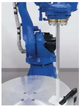
Today´s measurements of TCP transformations are often limited to manual processes. This is done with the help of specially designed tool tips (Fig. 1) that have to be fixed on the floor and/or mounted on the robot to calculate the transformation between the flange and the used tool tip. The robot programmer has to manually align the robot tool tip to the fixed tip and has to repeat this several times to calculate the tool position. The tool orientation cannot be calculated with this ‘tip to tip’ setup. In order to use also the orientation of the tool the user can either copy the frame orientation of the robot flange, or manually align a desired edge or plane on the tool to the fixed tip. This method is highly depending on the skills of the robot programmer and is very unreliable and often not applicable due to missing outer geometrical lines on the mounted tools. Especially the visual robot positioning used in [1] often is insufficient in terms of accuracy.
Figure 1. Industrial robot with calibration tip [2].
Many identification problems have been solved over the last years especially in the field of the use of camera systems in combination with robots. In this setup the classic hand-eye transformation is similar to the problem of determine an unknown TCP. Among others [3] describes the same identification problem that is used for TCP pose identification in the form of
. (1)
The unknown transformation describes the position and orientation between the camera frame and the robot wrist frame. In [3] the unknown transformation is solved with a geometric understanding and iterative solutions. This has many disadvantages. Neither exists a unique solution to the problem, nor is the orthogonality between the axes of the frame taken into account. Another
disadvantage is that the iterative solution is often time consuming.
III. ANALYTICAL ALGORITHM
The enhanced identification method introduced in this paper is based on an existing numerical, closed loop solution described in [4]. This method was developed to determine different gripper systems to mount voluminous structures [5]. Based on the relations shown in Fig. 2 the identification of the homogeneous transformation from the TCP to the flange coordinate system ( ) is realized. This is done by measuring the six degree of freedom pose of the TCP with an external measurement device ( ) and getting the corresponding flange transformation in respect to the robot base frame ( ).
Figure 2. Related coordinate systems.
A. Measurement of the TCP
A direct measurement of the TCP is often difficult to realize, because the tool frame is positioned on edges or geometries that are not accessible with external measurement devices.
Figure 3. Vector target holder for laser tracker tooling balls [6].
of freedom have to be determined a third tooling ball is attached near the TCP to generate a right hand coordinate system that lays in the origin of the TCP frame.
With three measured points ( ) two differential vectors are calculated and according to [7] used to create an orthogonal right hand coordinate system. The three points are determined with respect to the laser tracker coordinate system (x, y and z components). These point positions are used to derive the coordinate system attached to the TCP with its origin in the first point according to (2) - (4).
| | (2)
| | (3)
(4)
The resulting unit vectors define the rotational matrix of the homogeneous transformation, which is determined according to (5). Fig. 2 illustrates the necessity to determine this transformation in order to solve the problem of TCP identification.
(
)
(5)
B. Measurement of the Robot Flange
The third transformation in Fig. 2 represents the position and orientation of the robot flange with respect to the robots´ base coordinate system. The only possibility to directly derive this transformation is the robot controller. The controller calculates this information according to its kinematic model (forward transformation) and the measured joint values of each axis. During the identification process the robot controller is connected to the measurement computer and provides the pose of the robot flange frame.
C. Calculation of Unknown Transformation
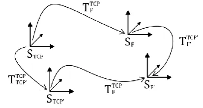
To calculate the transformation between according to [4] two independent robot movements have to be measured with all related coordinate systems shown in Fig. 2. The resulting new system of transformations after two robot movements is illustrated in Fig. 4.
Figure 4. Transformations related to two robot movements.
The transformation between the TCP and the robot flange is not changed during the movement. It is mechanical fixed to the robot flange so a simplification can be made according to (6):
(6)
The different transformations that are representing the constant transformation of the TCP to the robot flange can therefore be summarized to represent the unknown transformation according to equation (7):
(7)
To show the different components of the homogeneous transformations in Fig. 4 all transformations will be expressed according to (8) with separated rotational and translational components.
( ) (8)
( ) (9)
( ) (10)
( ) (11)
( ) (12)
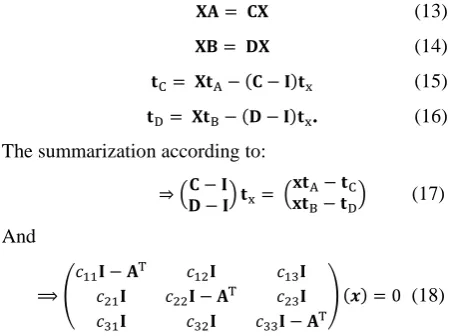
Extending the problem of (1) to two identification movements leads according to [4] eq. 6.21 to the different systems ( - unity matrix):
(13)
(14)
( ) (15)
( ) . (16)
The summarization according to:
( ) (
) (17)
And
(
) ( ) (18)
which leads to the numerical solution for two identification movements described in [4] equation 6.22:
(
)
IV. QUALITY CRITERIA
In order to compare different identification movements for the numerical solution described in (19) different quality criteria are used to evaluate the calculated transformation .
A. Conditional Number
The equation (19) is a linear equation system and can be simplified to the general form:
(20)
One quality criterion to solve the analytical problem of (19) is the conditional number of the system matrix in (20). The conditional number is an indicative value for the numerical accuracy of a system matrix and can be calculated with (21).
( ) ( )
( ) (21)
The investigation of the influence of the conditional number of the matrix of (19) for gripper identifications was previously discussed in [8].
B. Error Propagation
Equation (19) can be converted to the form of a direct function with the homogeneous translations related to the identification movements as input arguments (22).
( ) ( ) (22) The minimization of the function in (22) regarding error propagation in terms of the identified output also leads to two identification movements that differ from the movements derived from IV.A.
Both quality criteria were used in combination with a Powell minimization algorithm to calculate optimal identification movements. These existing movements that provide optimal error propagation and optimal conditional number were taken as reference identification movements for the numerical calculation according to (19) (see also V).
C. Field Check of TCP Transformation
Figure 5. Field check movement with calculated transformation .
In order to investigate a new optimal movement to calculate the unknown TCP transformation a third quality criterion is evaluated to interpret the resulting homogeneous transformation. Despite the quality
criterion of error propagation and conditional number (IV.A, IV.B) this quality criterion can be directly measured. It needs no use of minimization methods and is therefore suitable to be used as a field check that immediately derives the quality of the calculated transformation .
The related coordinate systems to interpret the quality of the transformation between the TCP and the robot flange with this field check are shown in Fig. 5. Here a movement of the TCP is expressed by a movement of the robot flange:
( ) (23)
where the homogeneous transformations can be expressed by
( ) (24)
And
(
). (25)
These transformations describe the relative movements of the TCP and the robot flange. To evaluate the quality of the constant transformation a movement around the TCP with no translational elements ( ( ) ) is executed by the robot flange according to (23). The deviation of the resulting position of the TCP is measured with the laser tracker in the TCP origin. With (24) and (25) the resulting TCP transformation can be described with the relationship
( )
(26)
In (26) the inverse transformation is used to calculate the new pose of the TCP coordinate system. To simplify the equations the pseudo-inverse of the homogeneous transformation is introduced in (27).
( ) ( ) ( ) (27)
The pseudo-inverse allows the multiplication of the matrix components in (26) and the individual presentation of the matrix components.
( ) ( ) ( ) (28)
( ( ) ) (29)
According to (26) the rotational and translational parts of the homogeneous transformation are:
(30)
mean distance between measured points is then calculated according to (32).
∑ ‖ ‖ (32)
The mean distance of the different measured positions can be used as geometrical quality criterion for the identified transformation .
V. NEW IDENTIFICATION MOVEMENTS
Several trials have shown, that the best identification results are achieved, when the rotational axes of the two independent identification movements are orthogonal to each other. Because of that a method was evaluated that creates an optimal second identification movement, depending on the first movement. For orthonormal rotational matrixes the rotational axes can easily be determined with (33).
( ) (33)
The eigenvector of the rotational matrix to the corresponding eigenvalue 1 ( denotes the unity matrix) is the rotational axis of . To directly calculate the components of (33) can be rearranged because of the orthogonally of the rotational matrix to
( ) (34)
This leads with the matrix components of
(
) (35)
To the components of the rotational axis
( ) (
) (36)
In order to create a second rotation axis with the rotational axis vector orthogonal to the first vector , the following equation is used:
( ) ‖( )‖ (37)
With this rotational axis and the relations from (36) the robot movement can be described according to the rotations around the three axis of the TCPs´ coordinate system , and . The roll pitch yaw convention [9] is used to derive the angles around the corresponding axes , and
( ) ( ) ( ) (26)
( ) ( )
(27)
( ) (
) (28)
( ) ( ) (29)
(
) (30)
1
In order to create a rotation that is to some degree predictable by the robot user the rotation described by the matrix was set to zero ( ), which leads to the resulting rotational axis representing the rotation around the axes of the flange coordinate system:
( ) (
) (31)
( ) (
) (32)
The resulting rotation about the flange axis can be determined using:
( ) (33)
( ) (34)
With these rotations and an orthogonal translation the homogenous transformation for the second identification movement can be calculated [10] and executed by the robot.
VI. APPLICATION EXAMPLE
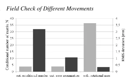
A. Field Check of Different Movements
Figure 6. Influence of different identification movements on field check.
The different ways to determine optimal identification movements described in IV.A, IV.B and V. were compared in terms of conditional number of matrix and the geometrical quality criteria described in IV.C. The result is shown in Fig. 6. Although the conditional number of the sytem matrix increases the RMS2 deviation of the field check decreases with orthogonal rotation axes and orthogonal translation vectors. According to previous observations this confirmes the suspicion that a low conditional number is a necessary
1
For reasons of compact layout a short form for cosine and sine was used: ( ) , sin ( )
but not sufficient quality criterion for accurate tool frame identification.
B. Milling Process
To illustrate the advantages of a reliable and accurate TCP determination an automated milling process is presented. To secure the comparability of all process parameters except of the transformation from TCP to robot flange ( ) remained unchanged. As a work object of the milling process an aluminium block was selected. During the process two pockets where cut into the aluminium (for process details see Appendix A). The process is illustrated in Fig. 7.
Figure 7. Robot pocketing process in aluminium block.
The first block was machined after a manual tip to TCP adjustment according to Fig. 8. The second block was machined after the automated measurements with two movements with orthogonal translation and rotation axes. With these movements the transformation between TCP and robot flange was calculated according to (19).
Figure 8. Manual tool calibration with external tip.
To compare the results of the two milling processes several points on the pocket surface where measured and the deviation according to a fitted plane evaluated. The results are shown in Fig. 9.
TABLE I. POCKET SURFACE AFTER PLANE FITTING
Trial No. No. of points
Deviation from fitted plane RMS
Deviation
Max Deviation (Signed)
Min Deviation (Signed)
1 7828 0.032580mm 0.075575mm -0.093020mm
2 5557 0.032054mm 0.081140mm -0.086972mm
Although the deviation from the fitted plane in Table I implies small differences between the two trials, the right picture in Fig. 9 shows a more homogeneous surface structure along the entire tool path. This corresponds with the optic and haptic quality impressions of the two blocks.
Figure 9. Surface of manually teached tool transformation (left) and automatically calculated tool transformation (right).
Especially on the diagonal connection lines from the centre to the corners of the pockets different surface qualities are visible (Fig. 10). The reason for this is the change of direction in the robot path during machining. In this region the effect of incorrect tool data can be presumed to be the highest.
Figure 10. Surface impression of teached tool transformation (left) and automatically calculated tool transformation (right).
To compare these regions the marked area in Fig. 10 was measured separately to demonstrate the effects of the different tool measurement strategies (Fig. 11).
Figure 11. Deviation of measured points along a diagonal line inside the two machined pockets.
In conclusion of the milling trials a higher continuity of the machined surfaces with automated measurement can be observed. It was shown that the manual teached tool transformation has a negative influence on the surface quality especially in regions with changing dynamical parameters.
VII.SUMMARY
measuring the unknown transformation from the robot flange to the tool centre point of a standard industrial robot. Former use of the algorithm was based on iterative computed relative movements based on minimized functions in respect of error propagation and conditional number. To compare the quality of the resulting transformation the paper introduced a field check method and the definition of a geometrical quality criterion. Based on the observed behaviour of the existing iterative computed relative movements the assumption was confirmed that relative movements with orthogonal rotational axes lead to the best results when determine the unknown tool transformation with two measured movements. To demonstrate the results a milling application was realized with the use of the developed method.
VIII.APPENDIX A PROCESS CONDITIONS
Equipment used during the milling processes is listed in Table II. The corresponding process parameters are shown in Table III.
TABLE II. EQUIPMENT USED FOR MILLING TRIALS
Type of Equipment Manufacturer Modell
Industrial robot ABB IRB 6660
HSC spindle SL SLQ120
Milling cutter Garant 20963510/10
Laser tracker target holders Leica Reflector holder 0.5”, offset 10mm
Laser tracker Leica AT901LR
Tooling balls Leica TBR 0.5”
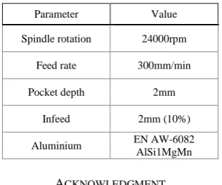
TABLE III. PROCESS PARAMETERS FOR MILLING TRIALS
Parameter Value
Spindle rotation 24000rpm
Feed rate 300mm/min
Pocket depth 2mm
Infeed 2mm (10%)
Aluminium EN AW-6082 AlSi1MgMn
ACKNOWLEDGMENT
The authors wish to thank Dr. Dirk Niermann for his support and valuable comments.
REFERENCES
[1] Roboterprogrammierung 1, 1st ed. KUKA Roboter GmbH,
Augusburg, Germany, 2011, pp. 57-67.
[2] Yaskawa Product Information, Yaskawa Europe GmbH,
Allershausen, Germany, 2014.
[3] Y. C. Shiu and S. Ahmad, “Calibration of wrist-mounted robotic sensors by solving homogeneous transform equations of the form AX = XB,” IEEE Transactions on Robotics and Automation, vol. 5, pp. 16-29, February 1989.
[4] P. Stepanek, K. Rall, and J. Wulfsberg, Flexibel Automatisierte Montage von Leicht Verformbaren Großvolumigen Bauteilen, 1st ed. Aachen, Germany: Shaker, ch. 6, 2007, pp. 56-76.
[5] J. Wollnack and P. Stepanek, “Bestimmung von montagekoordinatensystemen,” in Werkstattstechnik Online, Springer-VDI-Verlag, 2005.
[6] Product Brochure. (Jan 2014). Brunson Instrument Company. [Online]. Available: http://www.brunson.us/product-category/all- products/3-d-measurement-products/metrology-targeting-target- holders-kits-scales-bars-stands-mounts/metrology-smr-target-holders-adapters-kits-scale-bars
[7] J. Wollnack, “Determination of position and orientation from position information,” in Technisches Messen: tm, 2002, pp. 308-316.
[8] D. A. Valencia, “Study of a flexible prototype facility for large component assembly in aircraft manufacturing,” Diplom-Thesis, Institute of Production Management and Technology (IPMT), Hamburg University of Technology, Hamburg, Germany, 2013. [9] J. Wollnack. (2007). Skript Robotik. Analyse. Modellierung und
Identifikation. [Online]. Available: http://www.tu-harburg.de/ft2/wo
[10] R. N. Jazar., Theory of Applied Robotics, 2nd ed. US: Springer, 2010, ch. 2, pp. 33-90.
Christof Borrmann was born in Hildesheim (Germany) in 1981 and received his Dipl.-Ing. degree in mechatronics from the Hamburg University of Technology (Germany) in 2009. Currently he is working as a research project manager at the Fraunhofer Institute for Manufacturing Technology and Advanced Materials (IFAM) in Stade (Germany). His fields of research are industrial robot calibration, CAD/CAM systems, robot offline-programming and 3D measurement technology.