A variant of the look-down model with selection*

(1)

Boubacar Bah

1

Abstract. The goal of this paper is to study a new version of the look-down model with selection, where the population sizeN is finite and fixed. As in [1], we show (see Theorem 1.2) convergence in probability, locally uniformly int, as the population sizeN tends to infinity, towards the Wright-Fisher diffusion with selection.

Résumé. Dans ce papier on présente une variante du modèle étudié dans l’article [1]. On étudie le modèle du look-down avec sélection dans le cas d’une population de taille finie et fixée. Nous montrons que la proportion de l’un des types converge en probabilité, quand la tailleN de la population tend vers l’infini, vers la diffusion de Wright-Fisher avec sélection.

Introduction

The look-down model and the modified look-down model have been introduced by Donnelly and Kurtz (see [3] and [4]) to give the genealogical process associated to a diffusion model of population evolution. The idea is to distribute the population on sites indexed by i ≥ 1, with exactly one individual per site. This powerful representation is now currently used.

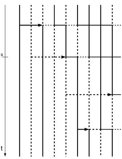
We briefly recall the definition of the modified look-down model, without taking into account any spatial motion for the individuals. Consider an infinite size population evolving forward in time. For any 1≤i < j, at rate one, the individual sitting on site i gives birth to an individual sitting on set j, and all individuals sitting on a site greater than or equal to j are shifted to the right (see Figure 1 ), that is to say each of those individual will move to the site which is at his right. These reproduction events involving levels i and j are called look-down events.

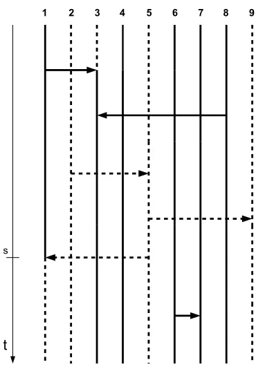
The two main differences between this model and the Moran model (see Figure 2), are that first, the arrows representing births are always pointing to the right, that is to say an individual sitting on sitei can only give birth to an individual on a sitej withj > i(The asymmetry which results from this choice is compensated by exchangeability, which is an important property of the look-down model). This ensures that the infinite model is well defined. Indeed, if we restrict ourselves to the firstN individuals, the evolution is determined by finitely many arrows. This would not be the case with the standard Moran model, which could not be described in the caseN =∞. In the Moran model with infinitely many individuals, there would be infinitely many arrows towards any individuali, in any time interval of positive length.

The second difference is that the individual who was sitting on the site where the offspring took place does not disappear, but instead is moved to the right, just as all the individuals which are on a site to his right.

∗ _{The author wish to thank an anonymous Referee, whose excellent and very detailed report permitted me to correct some}

imprecisions in an earlier version of this paper.

1 _{CMI, LATP-UMR 6632, Universit´}_{e de Provence, 39 rue F. Joliot Curie, Marseille cedex 13, FRANCE; [email protected]} c

EDP Sciences, SMAI 2014

(2)

t s

Figure 1. The graphical representation of a modified look-down construction. At timessthe

individual sitting on level 2 gives birth to an individual sitting on set 5. For all k ≥5, the individual at levelk is instantaneously shifted to levelk+ 1.

In [5], Donnelly and Kurtz added selection for a finite number of type individuals to their model, which involved additional births or possible deaths.

In our model, when a death occurs, the individual who dies is removed from the population, and each of the individuals sitting on a site to the right of his site are shifted to the left.

The aim of this paper is to present a variant of the model studied in [1]. We consider a population of fixed size N. We assume that two types of individuals coexist in the population : individuals with the wild-type alleleb and the individuals with the advantageous alleleB. This selective advantageous is modeled by a death rateαfor the typebindividuals, while the typeBindividuals are not subject to that specific death mechanism. We first recall the model from [1] withN =∞called (L∞_{), and then we will describe the variant which will}

be the subject of the present paper.

Look-down model with selection(called (L∞)) : We consider a population of infinite size. We will consider the proportion ofbindividuals. Hence typeb individuals are coded by 1, andB by 0. We assume that individuals are placed at time 0 on levels 1,2,...., each one being, independently from the others, 1 with probabilityx, 0 with probability 1−x, for some 0< x <1. For anyt ≥0,i≥1, letηt(i) denote the type of the individual sitting on site i at time t. Clearly ηt(i) ∈ {0,1}. The evolution of the population is governed by the two following mechanisms.

(1) Births. For any 1≤i < j <∞, arrows are placed fromito j according to a rate one Poisson process, independently of the other pairs i0 _{< j}0_{. Suppose there is an arrow from} _i _to _j _{at time} _t_{. Then a}

descendent (of the same type) of the individual sitting on leveliat timet− _{occupies the level}_j _{at time}

(3)

t s

Figure 2. The graphical representation of the Moran model of size N = 9. Arrows between

lines indicate resampling event. By resampling the genealogical relationships between individ-uals change. At times the individual at the level 5 gives birth to an individual who replaces the individual sitting on level 1.

(2) Deaths. Any type 1 individual dies at rate α, his vacant level being occupied by his right neighbor, who himself is replaced by his right neighbor, etc. In other words, independently of the above arrows, crosses are placed on each level according to a rateαPoisson process, independently of the other levels. Suppose there is a cross at level i at time t. If ηt−(i) = 0, nothing happens. If η_t−(i) = 1, then ηt(k) =ηt−(k) fork < i, andηt(k) =ηt−(k+ 1) fork≥i.

This model has been formulated by Anton Wakolbinger in an oral presentation [6]. Note that with those deaths, the infinite model is no longer immediately well defined, since for eachN ≥1, the evolution of the individuals sitting on the first N sites depend, in case of death, on the individual sitting on the following sites. Contrary to models defined in [3], [4], [5], the process YN

t = N−1(ηt(1), . . . , ηt(N)) is not a Markov process but it is approximately Markovian (see [1] fore more details). We can modify the model (L∞) as follows.

N-Look-down model with selection (called (N–L∞)) : For eachN, consider the process{η_tN(i), i≥1, t≥0}, obtained by applying only the arrows between 1≤i≤j ≤N, and the crosses on levels 1 toN. In other words, all arrows pointing to levels aboveN, and all crosses on levels aboveN have been erased. We then have a finite number of arrows and crosses on any finite time interval, and{ηNt (i), i≥1, t≥0}is constructed in an obvious way, by implementing the effect of the arrows and crosses, in the order in which they are met.

We are going to present now the variant of the look-down construction with selection called (LN_{), where the} sizeN ∈_N={1,2, . . . ,}of the population is finite and fixed. As in the model (L∞), we denote byζN

(4)

1 at levelN with probabilityaN(t), type 0 with probability 1−aN(t), whereaN(t) is the proportion of typebindividuals before the death eventt, see below.

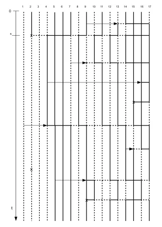
We can represent this evolution graphically, drawing the set [1, N]×R. A point (i, t)∈[1, N]×Rstands for the individual that occupies leveli at timet. Times goes from the top to the bottom. The jump times of the Poisson process associated to the pair (i, j),1≤i < j≤N are represented by arrows from itoj. We refer the reader to Figure 3 for a pictural presentation of our model.

We want to choose the type of theN individuals at time 0 in an exchangeable way, with the constraint that the proportion ofb individuals is given. One possibility is to draw without replacementN balls from an urn where we have putkred balls (which represent the type bindividuals) andN−kblack balls (which represent the typeB individuals). At each draw, each of the balls which remain in the urn has same probability of being chosen.

It follows from the above considerations and Proposition 3 in [1] that at each timet >0, the types of theN

individuals are exchangeable. Now, for eacht≥0, we define

X_tN = 1

N

X

i=1

ζ_tN(i), (0.1)

and iftis a death time

aN(t) = 1

N

X

i=1

ζ_tN−(i) =X_tN−.

The random variableX_tN ∈[0,1] represents the proportion of typebindividuals in the population.

In the next section, we prove that X_tN → Xt in probability, locally uniformly in t ≥ 0, where Xt is a [0,1]–valued Markov process, solution to the the stochastic differential equation

dXt=−αXt(1−Xt)dt+

p

Xt(1−Xt)dBt, t≥0,

where B is standard Brownian motion. From this, we compare our new model with the model from [1], i.e we compare the model (LN) with the model (L∞).

1. Convergence to the Wright-Fisher diffusion with selection

Recall the process{ηt(i), i≥1, t≥0}and{ζtN(i), i≥1, t≥0}defined in the introduction. LetN >2 denote a fixed integer, which will represent the size of the population in the model (LN_{). For each 1}_≤_M _≤_N₋_{2, we} define

X_tM,N = 1

M

X

i=1

ζ_tN(i),

and

Y_tM = 1

M

X

i=1

ηt(i).

X_tM,Nrepresents the proportion of typebindividuals at timetin the model (LN_{) among the first}_M _individuals, and YM

(5)

x

x x

t

Figure 3. The graphical representation of a modified look-down construction with selection

of size N = 17. The vertical time axis is shown on the left to the right, time flows from top to bottom. Solid lines represent type b individuals, while dotted lines represent type B

(6)

exists a stopping time ζ∞<∞a.s. such thatYζ ∈ {0,1}. That is to say one of the two types b orB fixates in

a finite time. To see this, we will look backwards from time t to time0. For eacht >0, we denote byZN

t the highest level occupied by the ancestors at timetof theN first individuals

at time0. For simplifying, we suppose that at time0the N first individuals are ofbtype. In this condition, the process(ZN

t )t≥0 is a jump Markov process with state space{1,2. . . ,∞}. When in staten, the process jumps to (1) n−1 at rate n₂

;

(2) n+ 1 at rate αn,α >0.

In other words, the infinitesimal generator of {ZN

t , t≥0} is given by:

QNf(n) =

_n

2

[f(n−1)−f(n)] +αn[f(n+ 1)−f(n)].

Now, let

ζN = inf{t≥0 :ZtN = 1}.

We first note that ZN

0 =N and ZζNN = 1. Clearly(ζN)N≥1 is increasing and limN→∞ζN :=ζ∞ is the time of fixation. One says that the model (L∞) comes down from infinity when the fixation timeζ∞ is finite.

We are going to show that ζ∞<∞a. s.Let

f(n) =

∞

X

k=n+1 1 k 2

−αk =

∞

X

k=n+1

2

k(k−1−2α).

For each n >2α,f(n)is well defined. In the next, we suppose thatn >2. We have

f(n−1)−f(n) = _n 1 2

−αn and f(n+ 1)−f(n) =

−1 n+1

2

−α(n+ 1)

Since n→1/ n₂−αnis decreasing, we obtain

QNf(n) = n 2 n 2

−αn−

αn

n+1 2

−α(n+ 1)

≥ n 2 n 2

−αn− αn

n 2

−α(n) = 1.

The processf(Z_tN)−f(N)−Rt

0Qf(Z N

s )dsis a martingale. The quantity ζN is a finite stopping time for each

N ≥1. Letk≥1, applying the optional sampling theorem to the bounded stopping time ζN ∧k, we get :

E(f(Z_ζN

N∧k)−E

Z ζN∧k

0

QNf(Z_sN)ds !

=f(N).

With the inequalityQN_f₍_N₎_≥₁ _{for some}_{N >}₂_α_{, we deduce that}

(7)

Theorem 1.2. Suppose that XN

0 →xa.s., as N → ∞, where 0< x <1. Then for all t >0 XtN →Xt a.s.,

where{Xt, t≥0} is a weak solution to the following SDE :

(

dXt=−αXt(1−Xt)dt+

p

Xt(1−Xt)dBt, t≥0,

X0=x, 0< x <1,

(1.1)

B is a standard Brownian motion. This diffusion is called the Fisher-Wright diffusion with selection.

Proof: We first compareXtM,N andYtM. We have :

Proposition 1.3. For any 1≤M ≤N−2 such that M2_≥₁₆_α₍_N_{+ 1)}_,

P ∃t >0 :XtM,N6=Y M t

≤(N+ 1)

₄_α₍_N_{+ 1)} M2

N−M ,

in particular as N → ∞, this probability tends to0if _MN →c, wherec is a constant.

Proof: For each i≥1,t >0, letξi,Nt denote the level on which the individual who was sitting on leveli at time 0 sits at time t, where the evolution corresponds to the model (N–L∞) defined in the Introduction (all arrows pointing to levels aboveN, and all crosses on levels above N have been erased). The process ξti,N takes its values in {1,2, . . . ,}. Each time there is a birth on a level smaller than or equal to ξ_ti,N− , ξ

i,N

t has a jump of size 1. Each time there is a death on a level smaller than or equal toξ_ti,N− , ξ

i,N

t has a jump of size −1. In other words,ξi,N_t follows the position of the individual who was sitting on leveliat timet= 0 until his possible death, then follows the position of his left neighbor if ξti,N ≥2, etc. We insist upon the rule that when this individual is killed, he is replaced by his immediate left neighbor. We have

{∃t >0 :X_tM,N 6=Y_tM}={∃1≤i≤M, t >0 such thatζ_tN(i)6=ηt(i)}

⊂ {∃i≥1,0≤s < tsuch that ξi,N_s > N, ξ_ti,N =M}

={∃1≤i≤N+ 1,0≤s < tsuch that ξ_si,N > N, ξi,N_t =M}.

In other words, in order to have XtM,N 6=YtM, for some t >0 , we need that at least one individual following the look-down model with selection (the model (L∞)) visits the levelM, after having visited the levelN+ 1, and the identity follows from the following monotonicity property : i < j ⇒ξi,N_t ≤ξj,N_t a. s. for allt >0. Consequently

P∃t >0 :X_tM,N 6=Y_tM≤

N+1

X

i=1

P∃0≤s < tsuch that ξ_si,N > N, ξ_ti,N =M.

We first show that for eachM2_≥₁₆_α₍_N_{+ 1)}_,

P ∃t >0 such that ξN_t +1,N =M

≤

₄_α₍_N_{+ 1)} M2

N−M

(8)

ρN,M_t ≤ξN_t +1,N, 0≤t≤τ_MN,

where

τ_MN = inf{t >0, ρN,M_t =M}.

Indeed, an individual starting fromN+ 1 at time 0 will always be at level higher than or equal toρN,M_t at time

t. Clearly

P(∃t >0 such thatξtN+1,N =M)≤P(τ N M <∞), hence (1.2) follows from

Lemma 1.4.

P(τMN <∞)≤

₄_α₍_N_{+ 1)} M2

N−M .

Proof: Let {Xn, n≥1} and {Yn, n≥1} be two mutually independent sequence of i. i. d. r. v.’s, theXn’s being exponential with parameterM(M+ 1)/2, theYn’s being exponential with parameterα(N+ 1). We have

P(τMN <∞)≤

∞

X

n=1

P(X1+· · ·+Xn> Y1+· · ·+Yn+N−M).

Indeed, for the processρN,M_t to reachM, we need an excess ofN+ 1−M deaths compared to the number of births. Now

P(X1+· · ·+Xn > Y1+· · ·+Yn+N−M) =P e M(M+1)

4 (X1+···+Xn−Y1−···−Yn+N−M)_>₁

≤ E

eM(M4+1)X1n _E_e−M(M4+1)Y1n+N−M

= 2n

_α₍_N_{+ 1)}

α(N+ 1) +M(M+ 1)/4

n+N−M

≤

8α(N+ 1)

M2

n

4α(N+ 1)

M2

N−M .

Summing fromn= 1 to∞yields the result, since

∞

X

n=1

₈_α₍_N_{+ 1)} M2

n

≤1, providedM2≥16α(N+ 1).

We can now conclude the proof of Proposition 1.3. We note that forM2≥16α(N+ 1), any 1≤i≤N+ 1,

P ∃0< s < tsuch that ξi,N_s =N+ 1, ξ_ti,N =M

≤

₄_α₍_N_{+ 1)} M2

(9)

The result follows.

We can now proceed with the

Proof of Theorem 1.2. Recall the definition ofYtM. We have shown in [1] that

Y_tM →Xt a.s., asM → ∞, (1.3)

whereXtis a [0,1]–valued Markov process which solution of (1.1). Now, we are going to show thatXtN →Xta.s. LetM =N−2. We have

|M X_tM,N−N X_tN |≤2.

From which, we deduce that

|X_tM,N−X_tN |≤ 4

M. (1.4)

The last assertion together with Proposition 1.3 and (1.3), implies that

X_tN →Xt a.s. The result follows.

We can in fact prove an additional property.

Corollary 1.5. For allT >0,

sup 0≤t≤T

|X_tN −Xt| →0in probability, asN → ∞.

Proof: Thanks to (1.4), it suffices to show that sup₀_≤_t_≤_T|X_tN−2,N−Xt| →0 in probability, as

N → ∞.

For anyN ≥3, we have

P sup 0≤t≤T

|X_tN−2,N−Xt|> ε

≤P∃0< t≤T :X_tN−2,N 6=Y_tN−2+P sup 0≤t≤T

|Y_tN−2−Xt|>

ε

2

.

The result follows from the Proposition 1.3 and Corollary 4 in [1].

References

[1] B. Bah, E. Pardoux, and A. B. Sow, A look-dow model with selection,Stochastic Analysis and Related Topics, L. Decreusefond et J. Najim Ed, Springer Proceedings in Mathematics and Statistics Vol22, 2012.

[2] P. Billingsley,Convergence of Probability Measures, 2d ed., Wiley Inc., NewYork, 1999.

[3] P. Donnelly and T.G. Kurtz. A countable representation of the Fleming Viot measure- valued diffusion.Ann. Probab.24, 698–742, 1996.

[4] P. Donnelly and T.G. Kurtz. Particle representations for measure-valued population models.Ann. Probab.27, 166–205, 1999. [5] P. Donnelly and T.G. Kurtz. Genealogical processes for Fleming-Viot models with selection and recombination,Ann. Appl.

Probab.9, 1091–1148, 1999. Wiley, New York, 1986.