27
THE IMPACT OF INDIRECT TAXES ON ECONOMIC GROWTH
Ana-Maria Uritescu, PhD student Bucharest University of Economic Studies
Email: ana.uritescu@fin.ase.ro
Abstract: This study analyzes the impact of indirect taxes on economic growth in Romania. Indirect taxes are represented by VAT and excise taxes. Annual data from 1993-1996 were used for the study. The data series consists of the weights of VAT in the GDP, the weights of excise duties in the GDP and the economic growth rate.
The link between the three data series is tested by the autoregressive vector technique and the Granger-causality. The results of the model indicate that there is a long-term relationship between VAT, excise duty, and economic growth. The Granger test results show that the data series represented by the weight of VAT in GDP and the data series represented by the weight of excise duties in GDP cause Granger growth rate.
Keywords: VAT, excise, economic growth, var, Granger causality
Introduction
Economic growth is a topical subject. It has been studied over time in various countries and mentioned in the speciality literature. Economic growth can be achieved through the correct management of fiscal and budgetary policy, either by controlling budgetary expenditures and budgetary revenue or through the efficient use of fiscal policy instruments.
In the theory of economic growth, there were three trends: the neoclassical theory of economic growth, the endogenous theory of economic growth and economic growth models in which fiscal and budgetary policy variables are integrated. 16
The models of economic growth that support neoclassical theory are those built by Ramsey (1928), Solow (1956), Swan (1956), Cass (1965), Koopmans (1965). The most important neoclassical models of economic growth are: a) the Solow-Swan model (1956), which states that the positive growth rate of income per capita is only possible through the continuous development of technology, the saving rate is constant; b) The Ramsey-Cass-Koopmans model asserts that the saving rate is determined by maximizing the utility of the representative household on the infinite horizon; c) the Diamond model refers to the fact that the economy at equilibrium behaves as in the first two models, but this model brings into question new aspects of economic growth-economies characterized by different initial conditions that can converge towards different balanced growth trajectories. 17
The endogenous theory of economic growth was sustained by Romer (1990), Lucas (1998), Aghion-Howitt (1992), Grossman-Helpman (1991). Endogenous growth theory explores how innovation and technical progress generates economic growth.
Barro (1990) is among those who have developed models of economic growth in which fiscal and budgetary policy variables are introduced. These variables are represented by taxes and public expenditures.
16 ASE Publishing House, Bucharest, 2011
28 The link between taxation and economic growth is a strong one. Fiscal policy instruments can have a positive or negative impact on economic growth. The most important indirect taxes are VAT and excise duties. The VAT was introduced in Romania in 1993, replacing the tax on the movement of goods, which had been levied up to this year, and the excise duties were introduced at the end of 1991.
VAT is an indirect tax charged on value added at each stage of production and distribution and not on the total value of the product or service performed.18
Excises are the special consumption taxes due to the state budget for certain products from the country and from import.19
The importance of these two indirect taxes is also due to the fact that they have been introduced for the purpose of harmonizing with the EU tax system.
Literature review
In the literature, studies focusing on the impact of taxation on economic growth had varied results. Some have led to the idea that fiscal policy has positive effects on economic growth, others have resulted in a negative influence of tax on economic growth. The variety and number of studies on the impact of taxation on economic performance are explained by the diversity of tax variables used to observe their influences on economic growth.
Paul Cahin (1995) develops an endogenous growth model that highlights the negative impact of public investment, public transfers and distortionary taxes on economic growth.
Helms Jay (1985) produces an econometric model whose results indicate that tax increases delay economic growth, demonstrating a negative effect and an inverse relationship between the two variables. Charles B. Garrison, Feng-Yao Lee (1995), in the study "The effect of macroeconomic variables on economic growth rates: A cross-country study" studies for the period 1960-1987 the impact of macroeconomic variables on economic growth. One of the findings of the study is that there is a negative effect of high marginal tax rates on economic growth.
Eric M. Engen and Jonathan Skinner (1996) conducted a study to highlight the impact of taxation on US economic growth. The paper's conclusions were outlined by studying the impact of tax cuts on economic growth and, at the same time, by studying at the micro level of the supplied labour, investment demand, and productivity growth. The obtained results show that there is very little influence on the growth rate in response to changes in marginal tax rates by 5 percentage points and average rates by 2.5 percentage points, but these small effects may have a cumulatively higher impact on the standard of living.
Richard Kneller, Michael F. Bleaney, Norman Gemmell (1998) analyzes fiscal policy and economic growth in OECD countries. The conclusion of the study is that distortionary taxes reduce
growth, and non-distortiona
-productive costs on growth. Thus, the study indicates an increase in growth due only to -productive government expenditures, not to non-productive expenditures. The study is made for 22 developed countries with data between 1970 and 1995.
18 d economic, financial, and fiscal implication on indirect taxes, Economic Publishig House,
Bucharest, 2001
19
29 Hubert G. Scarlett (2011) analyzes the impact of taxes on economic growth using quarterly data between 1990 and 2010 in Jamaica. According to this study, indirect taxation has a positive and significant impact on economic growth, while direct taxation has a negative long-term impact.
O. J. Ilaboya and C.O. Mgbame (2012) is conducting a study analyzing the impact of indirect taxes on economic growth in Nigeria. The results show a negative and insignificant relationship between indirect taxes and economic growth in that state.
Methodology of research
To study the impact of VAT and excise on economic growth, I created an econometric model using the autoregressive vector method and I tested Granger causality. The data used are from 1993 to 2016. I took them from the country reports provided by the International Monetary Fund. The data were processed in Eviews. Data series represented by VAT and excise duties consist of their weight in GDP, and economic growth is reflected in the real GDP growth rate.
The stages of identifying the link between VAT, excises and economic growth rates are: data analysis, testing the stationarity of time series, testing the cointegration of time series, creating the VAR model, testing Granger causality, interpretation of results.
Data series analysis
To analyze the three sets of data that I work with, I realized with the Eviews program both the graphical representation of the evolution of the three data series and the descriptive statistics. The following figures show the evolution in time of the economic growth rate, the weight of the VAT in the GDP and the evolution of the weight of excises in the GDP. Descriptive statistics of data give us the average, the standard variation, the minimum and maximum of the three data series.
Figure no. 1. Evolution of the
economic growth rate
Source: own processing using Eviews 9
Figure no. 2. Evolution of the VAT weights in GDP
30 Figure no. 3. Evolution of excise duties weights in
GDP
Source: own processing using Eviews 9
Table No. 1. Descriptive statistics of data series
GDP VAT EXCISE
Mean 2.862500 6.650000 2.795833
Median 3.900000 6.650000 3.050000
Maximun 8.500000 8.500000 3.700000
Minimum -7.100000 3.600000 1.400000
Std. Dev. 4.331765 1.332536 0.701848
Skewness -0.871473 -0.629283 -0.735767
Kurtosis 3.052337 2.413012 2.353615
Jarque-Bera 3.040597 1.928542 2.583229
Probability 0.218647 0.381261 0.274827
Observations 24 24 24
Source: own processing
From previous images we can see that for the data series of the economic growth rate the maximum was reached in 2008 with 8.5%, followed by the minimum of the data series in 2009 of -7.5%. These values correspond with the beginning of the economic crisis (2008) and the peak of this stage in the Romanian economy (2009).
For VAT, the lowest value was in the first year in which this type of tax was introduced at 3.6% in 1993 and the maximum of 8.5% in 2012.
The minimum amount of excise duty weight in GDP was reached in 1996, with a value of 1.4%, and the maximum value of 3.7% was reached in 1993 and 2015.
Testing the stationarity of the data series
Testing the stationarity of each series was performed with the tests: Augmented Dickey-Fuller and Phillips Perron. The results of applying the two test for data series are highlighted in the table below:
Table No. 2. Results of the Augmented Dickey-Fuller test and of the Phillips Perron test t-statistic 1% level 5% level 10% level Prob
ADF GDP 2.957523 3.752946 2.998064 2.638752 0.0542
ADF VAT 2.528740 3.752946 2.998064 2.638752 0.1220
ADF EXCISE 2.380119 3.752946 2.998064 2.638752 0.1578
31
PP VAT 2.528740 3.752946 2.998064 2.638752 0.1220
PP EXCISE 2.641300 3.752946 2.998064 2.638752 0.0995
Source: own processing
As the test results indicate, all three sets of data are non-stationary. The results of the t-statistical test must be higher than the values associated with the relevance levels for the stationarity of a data series.
The autoregressive vector technique is applied only to stationary data series. Thus, in order to create the econometric model, I applied the first difference for the three data series and I obtained the following results:
Table No. 3. Results of applying the first difference
First difference t-statistic 1% level 5% level 10% level Prob
ADF GDP 5.524476 3.769597 3.004861 2.642242 0.0002
ADF VAT 4.997455 3.769597 3.004861 2.642242 0.0006
ADF EXCISE 4.124990 3.769597 3.004861 2.642242 0.0051
PP GDP 5.823711 3.769597 3.004861 2.642242 0.0001
PP VAT 4.997455 3.769597 3.004861 2.642242 0.0006
PP EXCISE 8.658604 3.769597 3.004861 2.642242 0.0000
Source: own processing
As can be seen, the T-statistics value is superior to all values associated with the relevance levels. Thus, by applying the first difference, the three data series become stationary.
Testing the cointegration of time series
Before testing the stationarity of data series I applied the Johansen Cointegration test to check which autoregressive vector model I use. If the test results indicate that the data series are not cointegrated, then I will use the unrestricted VAR model.
Table No. 4. Results of the Johansen Cointegration test
Sample (adjusted): 1995 2016
Included observations: 22 after adjustments Trend assumption: Linear deterministic trend Series: GDP VAT EXCISE
Lags interval (in first differences): 1 to 1
32 According to this test, the data series are not cointegrated. Considering this result, I will apply the model of an unrestricted autoregressive vector.
Creating the VAR model and interpreting the results
The application of the autoregressive vector with five lags for the three data series (economic growth rate, VAT and excise) generates the following results:
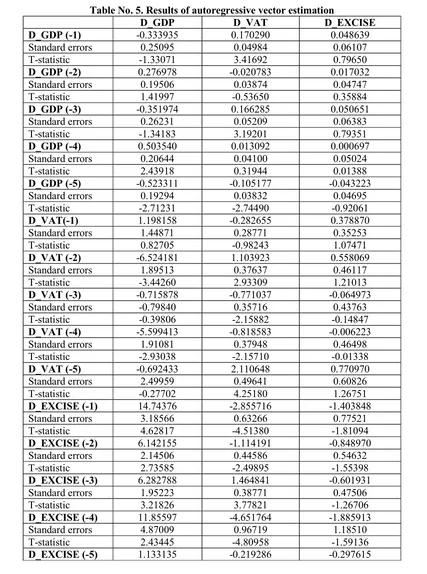
Table No. 5. Results of autoregressive vector estimation
D_GDP D_VAT D_EXCISE
D_GDP (-1) -0.333935 0.170290 0.048639
Standard errors 0.25095 0.04984 0.06107
T-statistic -1.33071 3.41692 0.79650
D_GDP (-2) 0.276978 -0.020783 0.017032
Standard errors 0.19506 0.03874 0.04747
T-statistic 1.41997 -0.53650 0.35884
D_GDP (-3) -0.351974 0.166285 0.050651
Standard errors 0.26231 0.05209 0.06383
T-statistic -1.34183 3.19201 0.79351
D_GDP (-4) 0.503540 0.013092 0.000697
Standard errors 0.20644 0.04100 0.05024
T-statistic 2.43918 0.31944 0.01388
D_GDP (-5) -0.523311 -0.105177 -0.043223
Standard errors 0.19294 0.03832 0.04695
T-statistic -2.71231 -2.74490 -0.92061
D_VAT(-1) 1.198158 -0.282655 0.378870
Standard errors 1.44871 0.28771 0.35253
T-statistic 0.82705 -0.98243 1.07471
D_VAT (-2) -6.524181 1.103923 0.558069
Standard errors 1.89513 0.37637 0.46117
T-statistic -3.44260 2.93309 1.21013
D_VAT (-3) -0.715878 -0.771037 -0.064973
Standard errors -0.79840 0.35716 0.43763
T-statistic -0.39806 -2.15882 -0.14847
D_VAT (-4) -5.599413 -0.818583 -0.006223
Standard errors 1.91081 0.37948 0.46498
T-statistic -2.93038 -2.15710 -0.01338
D_VAT (-5) -0.692433 2.110648 0.770970
Standard errors 2.49959 0.49641 0.60826
T-statistic -0.27702 4.25180 1.26751
D_EXCISE (-1) 14.74376 -2.855716 -1.403848
Standard errors 3.18566 0.63266 0.77521
T-statistic 4.62817 -4.51380 -1.81094
D_EXCISE (-2) 6.142155 -1.114191 -0.848970
Standard errors 2.14506 0.44586 0.54632
T-statistic 2.73585 -2.49895 -1.55398
D_EXCISE (-3) 6.282788 1.464841 -0.601931
Standard errors 1.95223 0.38771 0.47506
T-statistic 3.21826 3.77821 -1.26706
D_EXCISE (-4) 11.85597 -4.651764 -1.885913
Standard errors 4.87009 0.96719 1.18510
T-statistic 2.43445 -4.80958 -1.59136
33
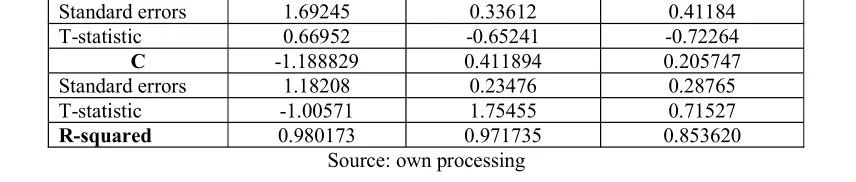
Standard errors 1.69245 0.33612 0.41184
T-statistic 0.66952 -0.65241 -0.72264
C -1.188829 0.411894 0.205747
Standard errors 1.18208 0.23476 0.28765
T-statistic -1.00571 1.75455 0.71527
R-squared 0.980173 0.971735 0.853620
Source: own processing
According to the results obtained by estimating the VAR model, we can see that the current GDP will increase on average by 0.33% if there is a 1% increase in the first-order GDP deviation, while the other variables remain constant. At the same time, for a 1% increase in second-order GDP delays, current GDP will increase by 0.27%. The sign of the coefficients for I, III and V delays indicates their negative impact on current GDP.
With regard to VAT, following the above table, it can be argued that for an I-time delay, a 1% increase in VAT in GDP generates GDP growth of 1.17% with a positive impact, but II, III, IV and V have a negative impact on GDP.
Regarding the impact of excise duties on GDP, it is noted that over time these have a positive impact on GDP.
R-Squared value of 0.980173% indicates a strong relationship between the three variables, but does not ensure that there is a positive link. In the long term, value added tax may have a negative impact on GDP and excise a positive impact.
Testing the Granger causality
After I estimated the autoregressive vector model, I tested Granger Causality for the three time series. Thus, I obtained the following results:
Table No. 6. Results of Granger Causality test Var Granger Causality/ Block Exogeneity Wald Tests
Sample 1993 2016
Dependent variable: D_GDP
Excluded Chi-sq df Prob.
D_ VAT 34.87858 5 0.0000
D_ EXCISE 43.75886 5 0.0000
ALL 78.51772 10 0.0000
Dependent variable: D_VAT
Excluded Chi-sq df Prob.
D_ GDP 23.91442 5 0.0002
D_ EXCISE 33.86408 5 0.0002
ALL 53.87555 10 0.0000
Dependent variable:D_ EXCISE
Excluded Chi-sq df Prob.
D_ GDP 1.398608 5 0.9245
D_ VAT 3.867868 5 0.5686
ALL 5.437190 10 0.8601
Source: own processing
34 of 0.0000 is inferior to the 5% relevance level, indicating that the null hypothesis is rejected and the assumption that D_VAT causes Granger GDP is accepted.
Concerning the link between excise duty and D_ GBP dependent variable, the probability value of 0.0000, below the 5% relevance level, indicates the rejection of the null hypothesis. This implied that excise duties (lag 1, lag 2, lag 3, lag 4, lag 5) do not cause GDP.
If D_VAT is the dependent variable it is obtained that D_GBP and excise duty cause D_VAT. The probabilities associated with the 0.0002 and 0.0000 test are below the 5% level and indicate the rejection of the null hypotheses. These assumptions assume that D_ GBP (lag 1, lag 2, lag 3, lag 4, lag 5) does not cause D_VAT and D_EXCISE (lag 1, lag 2, lag 3, lag 4, lag 5) does not affect D_TVA.
For the case where the data series of the share of excise duties in GDP is the dependent variable, the probabilities associated with the 0.9245 and 0.5686 tests lead to the acceptance of the null hypotheses. These null hypotheses assume that the GDP does not cause the excise duty and the VAT does not cause the excises because their values are biggest then relevance level of 5%.
Conclusions
The aim of this study was to analyze the impact of indirect taxes, represented by VAT and excises, on economic growth in Romania.
Using the technique of the unrestricted autoregressive vector I created an econometric model consisting of three data series: the economic growth seen through the economic growth rate, the VAT represented by the weight of VAT receipts in the GDP, and the third series was consisting of the excise duties in GDP. Annual data were between 1993 and 2016.
In the first part of the paper, I presented some studies on the same subject. The results of the studies were different, some highlighted a positive link, others a negative link between indirect taxes and economic growth.
The result of the study made by Richard Kneller, Michael F. Bleaney, Norman Gemmell in 1998 on Fiscal Policy and Economic Growth in OECD countries was that the distortionary taxes reduce the growth and the non-distortionary taxes don't.
According to Hubert G. Scarlett's 2011 survey for Jamaica, indirect taxation has a positive and significant impact on economic growth, while direct taxation has a negative long-term impact.
Following the application of the autoregressive vector method for selected data from our country, I have obtained that in the long run the VAT has a negative influence on the economic growth rate, and the link between the excises and the economic growth rate is a positive one.
The high value of R-Squared indicates the strong link between the three datasets.
In the last part of the work on the data series, the Granger causality test is applied. The most important result of this test is the one that indicates the influence that the two series of data, consisting of the weight of VAT in GDP and the weight of excises in GDP, have on the economic growth rate. The probability values associated with the 0.0000 and 0.0001 test points out that VAT and EXCISE are causing GDP.
Bibliography
[1] Charles B. Garrison,
Feng-growth rates: A cross- of Macroeconomics, vol. 17, Issue 2 pp. 301-317 [2]
35 [3]
4, pp. 617-642 [4]
543-559 [5]
MA, MIT Press [6] Ilaboya, O.J
[7] -Cross
and Statistics, Vol 67, issue 4, 574-82 [8]
-190
[9] ASE
Publishing House, Bucharest [10]
taxes, Economic Publishing House, Bucharest, 2001
[11] P. Cashin, (1995), Government Spending, Taxes and Economic Growth, IMF Staff Papers, vol. 42, issue 2, 237-269
[12]
-351 [13]
No. 5, Part 2
[14] Quarteley Journal of
Economic, Vol. 70, No. 1, pp. 65-94
[15] Government Spending in a Simple Model of Political Economy, Vol. 98, No. 5, Part 2
[16]
Issue 2, pp. 334-361
[17] onometric
Approach to Development Planning, Pontificae Academiae Scientiarum Scripta Varia, 28, 225-287, Amsterdam
[18] paper