J.-S. Dhersin, Editor
COLLECTIVE DYNAMICS AND SELF-ORGANIZATION:
SOME CHALLENGES AND AN EXAMPLE
Pierre Degond
1and S´
ebastien Motsch
2Abstract. In this review, we present an example of a system of collectively moving agents which exhibit spontaneous self-organization: this example consist of a model of ant-trail formation. We use this example to illustrate what are the challenges in the mathematical modeling of these systems and to outline some possible methodological tracks.
R´esum´e. Dans cet article de revue, nous pr´esentons un exemple de syst`eme d’agents en d´eplacement collectif qui d´eveloppe une auto-organisation spontan´ee: cet exemple consiste en un mod`ele de forma-tion de pistes de fourmis. Nous utilisons cet exemple pour illuster les d´efis se posant `a la mod´elisation math´ematique de ces syst`emes et pour proposer des pistes m´ethodologiques.
Introduction
Collective dynamics is observed in systems of a large number of agents moving coherently and forming swarms, flocks, schools, crowds, etc. The cohesion between the agents is maintained by interactions between neighboring agents, such as attraction or alignment. The cohesive interactions are local and the group does not have a definitive leadership. In spite of the local character of the interactions, these systems often exhibit large-scale structures, with time and length scales much larger than the typical agents’ interaction scales. The spontaneous appearance of large-scale structures which are not directly encoded into the agents’ interactions shows the ability of these system to produce ’self-organization’, a feature which has received the name of ’emergence’ in the literature. We refer the reader to the review [10] for examples and scientific issues related to collective dynamics.
Systems of a large number of interacting agents (or particles) can be described with various level of details. The models that provide the ultimate level of details are the ’Individual-Based Models (IBM)’, also called ’Par-ticle models’ in physics. They consist in following the position and state of each agent over time. They involve a large number of coupled ordinary or stochastic differential equations, which makes them computationally intensive. Additionally, they require some post-processing to give access to macroscopic observations, such as the system density, mean-velocity, order parameter, etc. Such post-processing may be highly non-trivial and affect the conclusions that can be drawn from the model.
A first level of coarse-graining consists in using a statistical description of the system, i.e. replacing the perfect knowledge of each agent’s position and state by a probabilistic description. The resulting models are
1 Universit´e de Toulouse; UPS, INSA, UT1, UTM ; Institut de Math´ematiques de Toulouse ; F-31062 Toulouse, France and CNRS; Institut de Math´ematiques de Toulouse UMR 5219 ; F-31062 Toulouse, France. [email protected]. Present address: Department of Mathematics, Imperial College London, South Kensington Campus, London SW7 2AZ, United Kingdom.
2 School of Mathematics and Statistical Sciences, Arizona State University, Tempe AZ 85287, USA. [email protected]
c
EDP Sciences, SMAI 2014
termed ’Kinetic Models’ (KM). In general, for an interacting particle system, it is not possible to obtain a closed equation for the probability distribution function of a given particle in position-state space unless a particular assumption named ’propagation of chaos’ is made. This is a statistical independence assumption on the particles which in general is true when the number of agents is large, although, in practice, it is often delicate to prove that such an assumption is actually satisfied. The KM in general consist of a single nonlinear integro-differential equation. Prototypes of KM are the Boltzmann and the Fokker-Planck equations.
The ultimate level of coarse-graining is to reduce the system description to a few macroscopic quantities such as density, mean velocity, order parameter, etc, as functions of position and time. The associated models are called ’Continuum models’ (CM) and consist of coupled systems of nonlinear partial differential equations. The derivation of CM from KM again involves some closure relation, i.e. ana prioriprescription for the dependence of the probability distribution function of the KM as a function of the state variables.
There has been an intense mathematical activity in kinetic theory to provide a rigorous framework to this hierarchy. We refer the reader to [4] for a review of these questions. Most of the literature deals with classical physics systems, such as rarefied gases, plasmas, semiconductors, etc. These theories should in principle be of great value to study self-organization in large systems of agents. Indeed, the emergence of structures at macroscopic scales calls for the use of CM. On the other hand, establishing a rigorous link between the IBM and CM levels (possibly through the KM level) is the only way to transfer any knowledge acquired at the macroscopic scale into a knowledge of the behavioral rules of the individuals, which is the ultimate target. Therefore, the use of kinetic theory methods seems the avenue to be taken.
Things are not so simple as the study of self-organization challenges kinetic theory in several ways. For instance, there are questions about the validity of the propagation of chaos in such systems. Indeed, self-organization is about the build-up of correlations between the agents: sampling the state of one agent randomly will give the state of the neighbouring agents with a high probability, which is clearly the sign of inter-particle correlations, which is basically the negation of any statistical independence of the particles. Indeed, we refer the reader to [2, 3] for an example of a system with breakdown of propagation of chaos. Here, in the first part of this paper, dedicated to ant trail formation, we will see another example of a system which probably (we are not able to prove it rigorously yet) exhibits the breakdown of the propagation of chaos.
Another question is about the passage from KM to CM, which in classical physics systems relies on con-servations (conservation of mass, momentum, energy etc.). Biological or social systems do not exhibit simple conservation relations. In [7], we have introduced the concept of ’Generalized Collision Invariant’ which provides a way to derive CM in situations where conservation relations are lacking. We refer the reader to the review [6] for a detailed account of this question and references. Here, in the second example of this note, we show how macroscopic models of crowds can be derived from an agent-based model of pedestrian behavior.
Finally, self-organization is intimately linked to phase transitions and hysteresis. Indeed, the same system in different conditions may exhibit different states of organization. For instance, according to the environment (such as the presence of predators), a school of fish may change from translational motion where all fish point in the same direction, into rotational motion, where the fish form a spinning mill. Additionally, when the initial environmental conditions are restored, the school may maintain its milling state, while it was in the directed state in the same condition before. This possible existence of two different self-organization states in the same environmental conditions and the dependence of the chosen state upon the history of the system is a characteristics of hysteresis phenomena. We refer the interested reader to the review [5] for a mathematical study of phase transitions in self-propelled particle systems, as well as references therein. Another kind of phase-transition is the so-called jamming phenomenon, in which a system of finite sized agents passes from a compressible phase to an incompressible one. The latter corresponds to a state where all agents are in contact to each other. This phase transition is observed in mammal herds for instance (see e.g. [8]).
1.
Ant-trail formation: motivation
This section is an abridged version of [1] with some new numerical simulations. Our goal is to model the transition from a continuum medium towards a network pattern. Many works are dealing with the dynamics of or on networks, but none of them (to our knowledge) has attempted to model this transition. For this purpose, the example of the formation of an ant-trail system has seemed to us one of the best examples of such a transition available in nature. Other applications could be for instance, the emergence of sheep paths in alpine pastures, or the formation of human trails in public environment [9].
Ants lay down signaling pheromones with their sting in a continuous fashion or in discrete streaks. In the last case, pheromone diffusion connects the neighboring streaks which have been deposited by the ant along with its motion. If plotted as a function of the two-dimensional spatial coordinates, the surfacic pheromone density resembles a hilly mountain ridge, with hill-tops at the deposition points. Ants can sense pheromone density gradients by sensing the concentration differences at the tips of their antennas. They turn towards the direction of higher concentration. This results in an undulatory motion about the crest of the mountain ridge. This mechanism is known as osmotropotactism. We refer to [1] for references.
In view of the previous description, it is legitimate to assume that ants lay down an information about the direction of their motion, namely the direction between two consecutive deposition points. We will take this observation as the starting point of our model. In a first step, we construct an IBM which assumes that agents moving with constant speed deposit information about the direction of their motion (which we will call a pheromone trail segment, of for short, a pheromone). An other agent passing by may, with a certain probability, decide to turn and align its motion with the direction of the trail segment. If several trail segments are available in the neighborhood, the agent chooses one of them at random. Trail segments have a finite lifetime and disappear after some time, thereby modeling pheromone evaporation.
After describing the IBM, we propose a KM and a CM based on this IBM. We will see that the KM and CM do not exhibit a transition to networks, as the IBM does. This questions the validity of the KM and CM as being approximations of the initial IBM.
2.
An IBM model of trail formation
Ants are described by their positionxi ∈R2 and their velocity direction ωi ∈S1 fori= 1, . . . , N whereN is the total number of ants. Likewise, pheromones are described by their positionxp ∈R2 and their direction
ωp ∈S1 forp= 1, . . . ,P where P =P(t) denotes the total number of pheromones, which can be a function of
time. Ants follow a random walk process. Between two velocity jumps, ants move in straight line at a constant speedc (the same for all the ants). This free motion is described by the differential equation:
˙
xi=cωi, ωi˙ = 0. (1)
We consider two types of velocity jumps: purely random ones and trail recruitment ones.
In the case of random velocity jumps, the direction of velocity after the jump differs from that before the jump by a random angle drawn out of a (periodized) Gaussian distribution with zero mean and variance σ2
. Jump times follow a Poisson process with given constant rate λr.
In the case of trail recruitment jumps, the velocity after the jump is drawn out of the pheromone directions
ωp of the pheromones located in ball of radiusR centered at the position of the considered ant. When several pheromones are present in this detection ball, one of them is selected at random with uniform probability. Two kinds of mechanisms can be envisioned: a polar one, where the ant velocity adopts the chosen pheromone direction, and a nematic one, where the ant velocity takes either plus or minus the pheromone direction, to make the jump angle acute. Trail recruitment jump times are selected according to a Poisson process whose parameter is proportional to the local pheromone density, i.e. the jump frequency is equal to λpMi(t) where
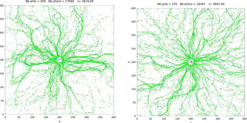
Figure 1. Trail system obtained with the IBM described above. Ants are released from the
center and leave the domain at the square boundary. Blue dots are ants. Green arrows are pieces of pheromone trails. Left: nematic interaction. Right: polar interaction. Closed loops are observed in the case of nematic interaction, but are not visible in the case of polar interac-tion.
recruitment more likely if there are more pheromones in some region. Some detection saturation mechanism could also be implemented by making the jump frequency a nonlinear function of the local pheromone density. Pheromones are deposited by the ants according to a Poisson process with rate νd. In this process, a new pheromone is created at the deposition time. This pheromone is located at the deposition location and its direction coincides with the direction of the ant velocity at the deposition time. Pheromones evaporate, i.e. they disappear according to a Poisson process of parameter 1/Tp, where Tp is the pheromone life-time. After deposition, pheromones remain immobile.
In [1], ants were initially located randomly with uniform spatial and orientation distributions. Simulations show that after an initial transient, a network of trails spontaneously emerges. It exhibits local persistence (i.e. the network topology is steady during a short period of time) and long-time plasticity (i.e. the topology changes drastically between two instants separated by a long period of time). Order parameters which quantify the transition from a uniform distribution to a network distribution of trails have been defined. The observations show that the transition occurs over one decade of variation of the parameters λp andλr. A network state is favored by either large values of λp or small values of λr. In this case, the trail width is smaller than in the converse situation, (either small values ofλp or large values ofλr.
3.
Mean-field and macroscopic ant trail models
In this section, we derive mean-field and macroscopic ant trail models based on the IBM described above. We start with the mean-field kinetic model
3.1.
Kinetic model
Let the ant distribution function beF(x, ω, t) and the pheromone particle distribution function beG(x, ω, t), forx∈R2
,ω ∈S1
and t≥0. These objects respectively describe the number density in phase-space (x, ω) of the ants and of the pheromones. The pheromone dynamics is modeled by the ordinary differential equation:
∂tG(x, ω, t) =νdF(x, ω, t)−νeG(x, ω, t), (2)
where νe = T−1
p and νd is the pheromone deposition rate already introduced in the previous section. The
first term at the right-hand side describes pheromone deposition by the ants, while the second one describes pheromone evaporation.
The ant distribution function follows the kinetic equation:
∂tF+c ω· ∇xF =Q(F). (3)
The right hand side models velocity jumps, i.e.
Q=Qr+Qp,
whereQr andQp respectively stand for random and trail recruitment jumps. Both operators are written
Qk(F)(x, ω, t) =
Z
S1
Pk(ω′→ω)F(x, ω′, t)−Pk(ω→ω′)F(x, ω, t)
dω′, (4)
wherePk(ω′→ω) is the jump probability andkstands forrorp. We note that
Z
S1
Qk(F)(x, ω, t)dω= 0, (5)
expressing that the number of particles does not change during the process. We postulate that the jump probabilitiesPk satisfy the detailed balance
Pk(ω′→ω)
Pk(ω→ω′) =
hk(ω)
hk(ω′), (6)
wherehk is the equilibrium. Using (6), we introduce:
Φk(ω′, ω) =
1
hk(ω)Pk(ω
′→ω) = Φ
k(ω, ω′),
and we have
Qk(F)(x, ω, t) =
Z
S1
Φk(ω, ω′) hk(ω)F(x, ω′, t)−hk(ω′)F(x, ω, t)dω′. (7)
we note that Φkis symmetric. Classically, the equilibria, i.e. the solutions ofQk(F) = 0 are given byF(x, ω, t) = ρ(x, t)hk(ω) with arbitraryρ.
For the trail recruitment process, the equilibrium distribution is given by
hp(ω) =g(ω) :=G(x, ω, t)
T(x, t) , T(x, t) =
Z
S1
where T is the local trail density. If we additionally postulate a polar and isotropic interaction, we get the expression:
Qp(F)(x, ω, t) =λpT(x, t) (ρ(x, t)g(x, ω, t)−F(x, ω, t)).
For random velocity jumps, we assume that the equilibrium is a uniform distribution
hr(ω) = 1 2π,
and that the jump probability is isotropic, which leads to:
Qr(F) =λr
ρ(x, t)
2π −F(x, ω, t)
.
3.2.
Macroscopic model
We first scale the system to dimensionless variables. Lett0, x0=ct0, ρ0, T0, be respectively units of time, space, ant density and pheromone particle density and introduce x′ =x/x0,t′ =t/t0, ρ′ =ρ/ρ0, T′ =T /T0,
F′=F/ρ0,G′=G/T0. We define:
¯
νd=νdt0, νe¯ =νet0
T0
ρ0
, λp¯ =λpt0, λr¯ =λrt0.
We assume thatt0is a macroscopic time scale and is very large compared to theλ−r1andλ−
1
p . Consequently,
we introduce:
ε= ¯1
λp =
1
λpt0
≪1, σ= λr¯¯
λp = λr
λp =O(1).
We also assume that ¯νd and ¯νeare of the same orders of magnitude and define
η= 1 ¯
νd =
1
νdt0
=O(1), κ= νe¯ ¯
νd = νe
νd =O(1).
In scaled variables, the mean-field kinetic model becomes:
η ∂tGε=Fε−κ Gε, (8)
ε(∂tFε+ω· ∇xFε) =Q(Fε), (9)
with
Q(F) = (Qr+Qp)(F) = (T+σ) (µ ρ−F), (10)
µ=T g+
σ
2π T+σ , g=
G
T, (11)
T =
Z
S1
G dω, ρ=
Z
S1
F dω. (12)
In [1], it is shown that the macroscopic model obtained in the limitε→0 is formally written as follows:
∂tρ+∇x· T
T+σj
= 0, (13)
η∂tT =ρ−κT, (14)
η∂tg= ρ
T σ T+σ
1
2π−g
wherej=R
S1g(ω)ω dω,denotes the flux ofg. Eq. (15) is a closed equation forg. Then,gcan be inserted into (13) to compute the evolution ofρ. The ant distribution functionf =µat all times (see (11).
Eq. (15) expresses the relaxation of g towards the isotropic distribution 1
2π. Therefore, in the large time
limit, there is no trail formation. Looking at the pheromone flux j, which is related to the orientational order parameter α=|j|/T (α∈[0,1]) we get
η∂tj =−ρ
T σ T+σj.
This equation shows that the direction of the local pheromone flux stays constant and its intensity decays to 0 ast→ ∞. Additionally, the ant flux is always proportional to and smaller than the pheromone flux. Therefore, it also converges to 0 for large times.
These results are in contradiction to what is observed at the level of the IBM and shows that the passage from microscopic to macroscopic models of collective motion may be non-straightforward. Here, we attribute this discrepancy to the fact that the propagation of chaos property may not be true, which invalidates the mean-field kinetic model as stated above.
4.
Conclusion
In this paper, we have given an overview of the questions posed by the modelling of collective motion and self-organization. Then, we have investigated a particular example, consisting of an Individual-Based Model of ant-trail formation. We have numerically demonstrated that this model develops the formation of an ant-trail system. On the other hand, mean-field kinetic and macroscopic versions of this model are provided. The large-time behavior of the macroscopic model does not show any formation of ant-trail, in contradiction to what is observed at the microscopic level. We attribute this discrepancy to the fact that this system does not satisfy the propagation of chaos property. Consequently, the mean-field kinetic model is invalid. Future work is devoted to the derivation of a valid mean-field kinetic model, which necessarily retains some of the correlations that lead to the breakdown of the conventional kinetic models.
References
[1] E. Boissard, P. Degond, S. Motsch, Trail formation based on directed pheromone deposition, Journal of Mathematical Biology, 66 (2013), pp. 1267-1301.
[2] E. Carlen, R. Chatelin, P. Degond, B Wennberg, Kinetic hierarchy and propagation of chaos in biological swarm models, Phys. D, appeared online.
[3] E. Carlen, P. Degond, B Wennberg, Kinetic limits for pair-interaction driven master equations and biological swarm models, Math. Models Methods Appl. Sci., 23 (2013) 1339-1376.
[4] P. Degond, Macroscopic limits of the Boltzmann equation: a review in Modeling and computational methods for kinetic equations, P. Degond, L. Pareschi, G. Russo (eds), Modeling and Simulation in Science, Engineering and Technology Series, Birkhauser, 2003, pp. 3-57.
[5] P. Degond, A. Frouvelle, J.-G. Liu, A note on phase transitions for the Smoluchowski equation with dipolar potential, Proceed-ings of Hyp2012 - the 14th International Conference on Hyperbolic Problems held in Padova, Italy, June 25-28 2012, AIMS, 2013, to appear. arXiv:1212.3920
[6] P. Degond, A. Frouvelle, J.-G. Liu, S. Motsch, L. Navoret, Macroscopic models of collective motion and self-organization, Proceeding of the S´eminaire Laurent Schwartz, Ecole Polytechnique, 2012, to appear. arXiv:1304.6040.
[7] P. Degond, S. Motsch, Continuum limit of self-driven particles with orientation interaction, Math. Models Methods Appl. Sci., 18 Suppl. (2008) 1193-1215.
[8] P. Degond, L. Navoret, R. Bon, D. Sanchez, Congestion in a macroscopic model of self-driven particles modeling gregariousness, J. Stat. Phys., 138 (2010) 85-125.