Reduced models for blood flow in curved vessels

Eric Canc`es & Jean-Fr´ed´eric Gerbeau, Editors DOI: 10.1051/proc:2005002

REDUCED MODELS FOR BLOOD FLOW IN CURVED VESSELS

S. Balbis

, L. Formaggia

, G. Pontrelli

and C. Guiot

Abstract. Flow in curved pipes has been intensively investigated and applications to arterial flow are relevant both in physiological and pathological conditions. A comprehensive survey of the work devel-oped over almost one century from experimental and modelling point of view is carried out. Despite its complex nature, the 3D curved flow can be modeled, under reasonable assumptions, accounting only for 2, or even 1, geometrical dimensions. A couple of different reduced models are presented and discussed here. Results of numerical simulations demonstrate the role of curvature in the formation of the secondary flow patterns and in the asymmetry of wall shear stresses. Both the above features can have important haemodynamical effects and clinical diagnostic velocimeters should be equipped with correction algorithms for the measurement bias induced by vessel curvature.

1.

_{Background and introduction}

The study of the flow in curved vessels begins with Dean (1927). He first wrote the Navier-Stokes equations introducing a proper coordinate system (where the constant radius of curvature of the duct center-line is denoted byRand the radius of the circular vessel isa, see Fig. 1), and showed that, provided a fully-developed laminar flow was considered, the equations could be parametrized by the ratioλ= a

R and the Reynolds number Re

only. Their combination D =Re√λ is called Dean number after him. Perturbative solutions at low D were worked out by Dean himself (1928), predicting the appearance of secondary flow and a deviation of the axial profile from the symmetric Poiseuille parabolic shape. Successively, experimental works were mainly intended to provide qualitative verification to his numerical results. Also the case of highDwas approached with analytical methods, by modelling separately the inner core and the boundary layer (Barua,1963; Mori and Nakayama, 1965 and Ito ,1969), but in spite of several successive numerical works the local structure of the flow and the shear-stress exerted on the walls of a curved vessel are not yet completely clear. Lyne, in 1970, extended the Dean solution to the case of oscillatory flow using the boundary layer approximation to investigate the linearized

Navier-Stokes equations for large values of the Womersley numberα=a r_ρω

µ , whereωis the circular frequency ρandµthe fluid density and viscosity respectively. His results showed the existence of a four vortex secondary flow system separable in two distinct regions: an inviscid core and a viscous boundary layer. Zalosh and Nelson (1973) expanded the relevant equations in power series of λ, allowing perturbative analytical solutions for the limiting cases of low and high frequency parameterα. Experimentally, Munson (1975) and Scarton et al (1977),

∗ _{This study was partly supported by the RTN Haemodel (S.B. and L.F. participation to Cemracs 2004) and by Bernoulli}

Center of Lausanne (grant to S.B., fall 2003) 1

University of Torino, Neuroscience Dep., C.so Raffaello, 30, 10125 Torino, Italy.

2

MOX, Mathematics Department, Politecnico di Milano, Italy.

3

Istituto per le Applicazioni del Calcolo - CNR, Viale del Policlinico, 137, 00161 Roma, Italy. c

EDP Sciences, SMAI 2005

using dye filaments, were able to verify theoretical expectations at boundary layer. Some years later, Mullin and Greated (1980) worked out a parallel analysis expressing the solutions by means of finite Hankel integral transforms. Unsteady flow with a non-zero mean was investigated by Smith (1975) and more recently by Wang and Tarbell (1995). Fluid-structure interactions are important when considering physiological applications and compliant vessels. Many papers investigated this topic: for instance, Chandran and al. (1974) carried out the numerical solution of the linearised Navier-Stokes equations for an elastic curved pipe. Pedrizzetti (1998) studied the fluid flow in a tube with an elastic membrane insertion and recently, in 2001, Myers and Capper worked out the analytical solution for the axial velocity component in a curved elastic pipe, the case of unsteady flow in a curved vessels with variable curvature was investigated by Waters and Pedley (1999). A recent book presents a number of studies concerning biomedical wall-fluid interaction problems (Collins et al., eds. 2004). Finally, in these last years, many different experimental methods have been applied to verify theoretical expectations: Laser photochromic velocity techniques were applied by Park et al (1999) to investigate axial and radial velocities at

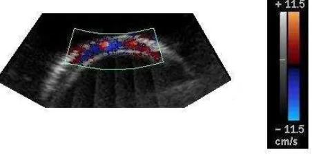
Re= 250 and Particle Imaging Velocimetry (PIV) has been used to investigate 3D velocity in a model of 90-degree bifurcation of square tubes (Nikolaidis et al, 2002). Since Doppler velocimetry is currently employed to assess circulatory disorders in large blood vessels, mainly in the head and neck district and in the limbs, Balbis et al (2004) used it to quantify diagnostic errors on curved vessels.In spite of the relevance of curvature in many vascular systems (aortic arch, coronary and umbilical vessels, etc), the bias due to vessel curvature had not been taken into consideration before 1999 (Guiot et al, 1999) among the many other well known factors which severely affect measurements accuracy (Gill, 1985). Blood vessel curvature is responsible for the appearance of nonaxial velocity components and for minor changes in the pattern of the axial flow and it can play an important role when considering the ”Doppler” examination of vessels (see Fig. 2). In principle, although nonaxial velocity components do not contribute to the overall blood flow along the vessel, their presence may cause flow over- or under-estimation when using a Doppler device. In addition to the bias due to nonaxial velocity components, the spread of the axial direction within the sample volume was investigated as well (Balbis et al, 2005), showing that the maximal velocity estimated by the Doppler probe and all related parameters, such as the shape of sonograms, strongly depend on curvature, while the mean velocity is generally less affected.

The previous experimental considerations show the influence of curvature in clinical applications and in diagnostic. The predicting capabilities of mathematical modelling is testified by the great deal of work developed during many decades (see above). Such a variety of models offer several advantages over the experiments and face the physical phenomenon from different points of view. Despite the flow complexity and the three-dimensional nature of the problem, models of lower degree of complexity (reduced models_{) can be developed: although defined}

on a limited number of variables they are fairly accurate and allow a noticeable computational saving.

2.

_{Mathematical modelling}

2.1.

A rigid wall model

One dimensional models are quite suitable for studying blood flow in arterial systems because of their computational efficiency. The first application of these models to the circulatory system dates back to the eighteenth century, with a first work of Euler (1775) and many other following papers. Recently, new impulses in this direction were given, for instance, by Sherwin et al (2001), Formaggia et al (2002) and Robertson and Sequeira (2004), who described blood flow in arteries using 1D models.

Starting from the theory of Cosserat curves, Green and Naghdi (1993) developed a general framework to study the problem of flow simulation on straight and curved cylindrical tubes. Given a generic domain with (x, y, χ) as coordinate system, beingx andy the cartesian coordinates on the plane of the vessel cross section andχthe axial direction, fluid velocity can be expanded on a suitable basis of shape functionsβ_n(x, y):

v(x, y, χ, t) = N

X

n=0

β_n(x, y)ωn(χ, t)

In principle, the accuracy of these models can be improved as desired by increasing the dimension of the basis of selected shape functions (in our case, polynomial functions), but numerical difficulties and computational constraints arise in practice, when the number of unknowns is too large. We have considered the problem of a time-dependent flow of an incompressible viscous fluid in a curved vessel with rigid walls and constant radius of curvatureR.

A very simple model assumes the following expansion for the velocity and pressure,

vχ=

1−x 2_+y2

R2

(a(χ, t) +c(χ, t)y) vx= 0,

vy=

1−x 2_+y2

R2

(e0(χ, t) +e2(χ, t)y), p=P0(χ, t) +P2(χ, t)y.

We are neglecting variation of velocity on thex direction. This reduces the problem to six equations in six unknowns: three of them can be estimated by considering the weak form of the Navier-Stokes momentum equations for uχ and uy and of the mass conservation divv = 0 (see eqn. (2)), while the remaining three equations can be obtained from the first order momentum of the same Navier-Stokes equations. Our model differs from the original one of Naghdi and Green because the divergence constraint is imposed in a weak (integral) form, which is allowed provided a dominant longitudinal component of velocity is assumed.

In order to improve the readibility of the results, we define the following new variables:

Q(χ, t) =π 2R

2_{a(χ, t),}

G(χ, t) = π 12R

4_{c(χ, t),}

F0(χ, t) = π 2R

2_{e0(χ, t),}

F2(χ, t) = π 12R

4_{e2(χ, t).}

The first is the volumic flux along the tube. The others are linked to the loss of symmetry of the velocity profile and the transversal component of the velocity, respectively.

¿From the continuity equation we get ∂Q

∂χ = 0, as expected being the tube rigid and with constant section.

This translates in the fact thatQis a function of time only. The satisfaction of the continuity equation imply also that ∂G

∂χ =F0+ 1

CF2, which acts as a contraint on the differential problem derived from the averaging of the momentum equation. The latter reads

                                                   dQ dt + 1 C ∂G

∂t + 6π ∂ ∂χ

G2

A2 +A

∂P0 ∂χ + 1 C A2 4π ∂P2

∂χ =−8πν Q A−

1

C24πν G A, ∂G ∂t + 1 C A 6π dQ

dt + 2 Q A ∂G ∂χ + 1 C A2 4π ∂P0 ∂χ − 1 C F2Q

A −6π F2G

A2 +

−4₃QF_A0 −_C1GF_A0 +A 2

4π ∂P2

∂χ =−24πν G A −

1

C3νQ,

∂F0

∂t +

1

C ∂F2

∂t + 6π ∂ ∂χ

GF2

A2 + 4 3

Q A

∂F0

∂χ +AP2=−8πν F0

A −

1

C24πν F2 A, ∂F2 ∂t + 1 C A 6π ∂F0 ∂t + Q A ∂F2 ∂χ − 1 C2 F0F2

A −

4 3

F2 0

A −6π F2

2

A2 +

∂ ∂χ GF0 A + 1 C A2 4πP2=

=−24πνF2 A −

1

Here,A=πR2 _{and C are the (constant) cross section area and the curvature of the tube, respectively. If we} impose the flux, we may assume that Q=Q(t) and ˙Q= dQ_dt are given functions. Under this hypothesis and after some tedious mathematical manipulations we may write the previuos system in the following form

              

∂G ∂t +

h

GF(F~) +σG

i

G+σF(F~) +A24π

∂P2

∂χ =RQ(Q,Q˙), ∂G

∂χ =F0+

1

CF2 ∂ ~F

∂t +M(Q, G) ∂ ~F ∂χ +

h

CF(F~) +BF

i ~

F =~bPP2.

where F~ = [F0, F2],K1, GF,σF, RQ, are given functions and σG is a constant, while M, CF andB are 2×2 matrices and~bP a given vector. All these quantities depend parametrically onAandC, and their expression is not reported here for the sake of space.

We may note that the constraint given by the second equation (resulting from the weak imposition of continuity) is counterbalanced by gradient of P2. Indeed the latter acts as a Lagrange multiplier. Finally, the last line is a system of two transport equations forF~.

The average pressureP0may be eventually recovered through

AC∂P0

∂χ +k2G=RG(Q),

beingRG another given function.

This system is highly non linear and the first attempts to solve it numerically has shown that it does not lend itself to a staggered treatment. Its numerical treatment is still under study as well as its analysis.

2.2.

An elastic thin-walled model

Wall compliance and fluid-wall interaction constitute an essential aspect in arterial flow that cannot be disregarded when considering wave propagation phenomena. In this section another possible reduced model for a blood flow through a curved thin-walled artery is presented.

The fluid flow is approximated by the Navier-Stokes equation:

ρ

∂v

∂t +v· ∇v

=−∇p+µ∆v (1)

with v the velocity andpthe transmural pressure. The fluid incompressibility reads as:

divv = 0 (2)

Due to the small thickness, the wall motion is described by the membrane theory. This is a thin shell subject to the inertial, elastic and fluid stress forces. The balance equation for fluid-wall system is:

divS =−p·n+ 2µD_·n+ρwu¨ (3)

whereS is the membrane stress tensor (with a linear shear-stress relationship), D is the rate of deformation tensor of the fluid, uthe wall displacement andρw the wall density (all the vectors at the r.h.s. are projected on the wall). Matching of velocities is imposed as interface fluid-wall condition:

Because of the geometry of the problem, a toroidal coordinate system (r, ψ, θ) is considered. It is well known that the vascular flow can be decomposed in a steady dominant part and, due to the wall compliance, in a small oscillatory component over it [17]. As a consequence, it is reasonable to look for an unsteady solution having the form of a longitudinal wave, superimposed on the steady solution, namely:

X = ¯X(r, ψ) + ˜X(r, ψ)ei(ωt−kz) ₍₅₎

(X denotes the global solution) whereω is the circular frequency,kthe wave number andz=R θa curvilinear axial coordinate. This allows to reduce the physical dimensions of the problem.

To simplify the mathematical problem, let us assume the unsteady part issmall_{enough such that the response}

of the system can be linearized, with respect to the wave amplitudes, over the steady state solution.

A perturbation method is used to study the influence of a moderate curvature with respect to the straight case. As the curvature parameterλis assumed to be small (1), the tilded quantities ˜X (amplitudes) in Eqs. (5) are expanded as a power series ofλover an axisymmetric solutionX0. By omitting∼sign at the right hand side, we have:

˜

X =X0+λX1+λ2X2+... (6)

In the asymptotic expansion Eq. (6),X0 corresponds to the axisymmetric solution in a straight elastic tube (Womersley solution) [33]. By equating the 1st order terms in the governing Eqs. and separating components of velocity and pressure as follows:

u1= ˆu1sinψ v1= ˆv1cosψ

w1= ˆw1sinψ p1= ˆp1sinψ (7)

the problem reduces to a system of linear ordinary differential equations (by omitting the circumflex accent):

du1

dr + u1

r − v1

r −ikaw1=fc(X0) d2_u

1

dr2 + 1

r du1

dr − ₂

r2 +iα 2

u1+

2v1

r2 −

a µ

dp1

dr =fu(X0) d2_v

1

dr2 + 1

r dv1

dr −

2

r2 +iα 2

v1+2u1

r2 −

ap1

µr =fv(X0) d2_w

1

dr2 + 1

r dw1

dr − ₁

r2+iα 2

w1+

ika2

µ p1=fw(X0) (8)

where a dimensionless radial variabler→r/ahas been used andαis the Womerseley number. Similar variable separation for displacements and first order scalar equations are written for the wall motion (3) and the fluid-wall interface matching conditions (4). Because of the continuity of the physical variables atr= 0, the following boundary conditions are imposed in the origin:

u1(0) =v1(0) u01(0) =v10(0) = 0 p1(0) =w1(0) = 0 (9)

3.

_{Numerical results}

The wave solution is then reassembled as:

X= ¯X+|X˜|cos ωt−Re(k)z+φ

exp(Im(k)z) (10)

withφ=arg( ˜X) (see Eq. (5)). It follows that all the variables have an oscillatory evolution in time, superim-posed over the steady state solution, with amplitude|X˜| and a phase lead or a phase lagφ. Both amplitude and phase are independent of time, while the amplitude has a damping factor given byexp(Im(k)z).

The physical problem depends on a large number of parameters, each of them may vary in a quite wide range, and there is an enormous number of different limiting cases. In the present work we will focus the attention on the influence of curvature – parametrized byλ– and letting all the others fixed.

In the simulations, we take the following numerical parameters, referred to the vascular flow in a medium sized arterial segment:

ω= 2π s−1 a= 0.5cm h= 0.05cm E= 107dyne/cm2 µ= 0.04g cm−1s−1 ρ=ρw= 1g/cm3 σ= 0.5

A= 26000dyne/cm2 dp¯0

dz = 7dyne/cm

3

The mesh size has been taken as ∆r= 0.02cm.

A cross section of a curved tube with the inner wall at the left side is considered (Fig. 1). Eq. (10) is used to plot the flow pattern, the pressure distribution and wall deformations for a given time (t = 0) and a fixed axial coordinate (z= 0).

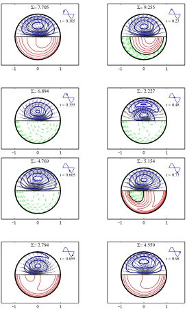
The effect of the curvature is examined by lettingλvary asλ= 0,0.05,0.1, and the correspondent amplitudes of the unsteady solution X0+λXˆ1 are depicted in Fig. 3. Note that in a curved tube the solution becomes asymmetric and the degree of skewness increases withλ. The structure and the evolution of the secondary flow is shown in Fig. 4. For the values of the parameters considered, a single vortex appears at most times, but a second vortex detaches from the wall and develops at the end of each half-cycle in the opposite direction. The strength of the secondary motion is measured through the index Σ = max

r,ψ

p

(Reu˜)2_{+ (Re˜v)}2 _(maximum

modulus of the cross section velocity). Axial velocity peak is shifted alternately inwardly and outwardly, and a reversal flow takes place at some instants.

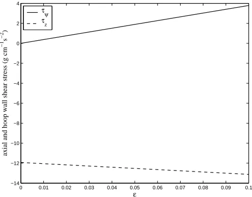
The amplitudes of the two components of the wall shear stress are obtained from the flow field as:

˜

τψ= ˜τψ0+λτ˜ψ1 =λ˜τψ1=

µλ a

ˆ

u1+dˆv1

dr −ˆv1

r=1 cosψ

˜

τz= ˜τz0+λτ˜z1=

µ a

_dw˜

0

dr +λ _dwˆ

1

dr −wˆ0

sinψ

r=1

It follows that the circumferential stress ˜τψ is present only in a curved tube and varies over a zero mean. On the other hand, the axial wall shear stress ˜τz varies over the correspondent value for the straight tube ˜τz0and its extrema are attained atψ=±π

2. Both of them vary linearly withλ, are opposite in sign, and the magnitude of the ˜τψ is smaller than ˜τz (Fig. 5).

Similarly to all the flow variables, the wall displacements are trigonometric functions of ψ (see Eq.(7)): as consequence|η˜|and|ζ˜|are maximum atψ=±π

4.

_Conclusions

The present investigation focuses on the relevance of curvature in vessels and on the possible different mod-elling approaches. In particular conditions, the elasticity of the vessel wall can be neglected, and a 1D reduced model is applicable. This approach is highly convenient and cheap, with respect to the more complex 2D and 3D models. Since such a model is expected to retain the main effects induced by the curvature on the fluid velocity, a possible application is that of estimating the errors produced by traditional (curvature-neglecting) clinical Doppler equipments in arterial diagnostics. In principle, a cost and time-effective algorithm could be implemented on clinical equipments: provided vessels dimension and curvature are extracted by Ultrasound imaging, a specific computation could be performed which almost in real time corrects the Doppler estimations of blood velocity and pulsatility. Work is in progress for optimizing such 1D reduced models and results are expected shortly.

In other vascular districts, the flow-vessel interaction cannot be disregarded, and another strategy for reducing complexity is possible. An asymptotic analysis can be carried out whenever the vessel radius is small compared to the radius of curvature, as is generally true in the human vascular system. Such an approach, which allows to treat fluid flow and wall mechanics simultaneously, would be very promising for understanding the influence on the wave propagation and the effects of the blood shear stress on the vascular endothelium in realistic curved arteries.

References

[1] S. Balbis, C. Guiot, S. Roatta, R. Arina, T. TodrosUltrasound Med. Biol.,30, 5, 639 (2004). [2] S. Balbis, S. Roatta, C. GuiotUltrasound Med. Biol.,31, 1, 65 (2005).

[3] S.N. Barua,Q.J.Mech.Appl.Math.,16, 61 (1963).

[4] S.A. Berger, L. Talbot and L.S. Tao,Ann. Rev. Fluid Mech.,15, 461 (1983).

[5] K. B. Chandran, W. M. Swanson, D. N. Ghista and H. W. Yao,Ann.Biomed. Eng.,2, 392 (1974).

[6] M. W. Collins, G. Pontrelli, M.A. Atherton (Eds),Wall-fluid interaction in physiological flows, Adv. Comput. Bioengin., 6, WIT Press (2004).

[7] W.R. Dean,Phil. Mag.,4, 208 (1927).

[8] C.A.J. Fletcher,Computational techniques for fluid dynamics, Vol.I, Springer-Verlag (1997). [9] L. Formaggia, D. Lamponi and A. Quarteroni,J. Engr. Math., submitted (2002).

[10] Y.C. Fung,A first course in continuum mechanics, Prentice Hall Inc. (1977). [11] R. W. Gill,Ultrasound Med. Biol.,11, 625 (1985).

[12] A. E. Green and P. M. Naghdi,Phil. Trans. R. Soc.Lond. A,342, 525 (1993).

[13] A. E. Green, P. M. Naghdi and M. J. Stallard,Phil. Trans. R. Soc.Lond. A,342, 543 (1993). [14] C. Guiot, S. Roatta, E. Piccoli, F. Saccomandi, T. Todros,Ultrasound Med. Biol.,25, 1465 (1999). [15] H. Ito,Z. Angew. Math. Mech.,49, 653 (1969).

[16] W. H. Lyne,J. Fluid. Mech.,45, 13 (1970).

[17] W. R. Milnor,Hemodynamics, 2nd ed., Williams and Wilkins,C8(1989). [18] Y. Mori and W. Nakayama,Int. J. Heat Mass Transfer,8, 67 (1965). [19] T. Mullin and C. A. Greated,J. Fluid. Mech.,98, 397 (1980). [20] B. R. Munson,Phys. Fluids,18, 1607 (1975).

[21] L.J. Myers and W.L. Capper,IEEE Trans. Biomed. Engin.,48, n. 8, 864 (2001). [22] H. Park, J. A. Moore, O. Trass, M. OjhaExperiments in Fluids,26 (1-2), 55 (1999).

[23] T.J. Pedley,The fluid mechanics of large blood vessels,Chapt. 4, Cambridge Univ. Press (1980). [24] G. Pedrizzetti,J. Fluid. Mech.,375, 39 (1998).

[25] G. Pontrelli and A. Tatone,Wave propagation of a fluid flowing through a curved thin-walled elastic tube, submitted (2004). [26] A. Robertson and A. Sequeira,A direct theory approach for modeling blood flow in the arterial system: an alternative to

classic 1D model, submitted (2004).

[27] H. A. Scarton, P. M. Shah and M. J. Tsapogas,Mechanics in Engineering, 111, University of Waterloo Press (1977). [28] S. Sherwin, L. Formaggia, J. Peir´o,Proceedings of ECCOMAS CFD 2001, CD-ROM Edition.

[29] F. T. Smith,J. Fluid. Mech.,71, 15 (1975).

[30] K. Sudo, M. Sumida and R. Yamane,J. Fluid. Mech.,237, 189 (1992). [31] D. M. Wang and J. M. Tarbell,J. Biomech. Eng.,117, 127 (1995). [32] S. L. Waters and T. J. Pedley,J. Fluid. Mech.,383, 327 (1999). [33] J.R. Womersley,Phil. Mag.,46, 199 (1955).

R

ψ

θ a

Figure 1. Cross section of the tube (inner wall at the left, outer wall at the right) and toroidal coordinates (r, ψ, θ).

−1 −0.5 0 0.5 1 −0.5

0 0.5 1 1.5 2

u 0

+

ε

u 1

(cm s

−1

)

−1 −0.5 0 0.5 1

−4 −3 −2 −1 0 1 2 3

v 0

+

ε

v 1

(cm s

−1

)

−10 −0.5 0 0.5 1

10 20 30 40 50

y

w 0

+

ε

w

1

(cm s

−1

)

−1 −0.5 0 0.5 1

2.595 2.6 2.605x 10

4

y

p 0

+

ε

p 1

(dyne cm

−2

)

−1 0 1

t = 0.105

Σ= 7.705

−1 0 1

t = 0.23

Σ= 9.255

−1 0 1

t = 0.355

Σ= 6.894

−1 0 1

t = 0.48

Σ= 2.227

−1 0 1

t = 0.605

Σ= 4.769

−1 0 1

t = 0.73

Σ= 5.154

−1 0 1

t = 0.855

Σ= 2.794

−1 0 1

t = 0.98

Σ= 4.559

0 0.01 0.02 0.03 0.04 0.05 0.06 0.07 0.08 0.09 0.1 −14

−12 −10 −8 −6 −4 −2 0 2 4

ε

axial and hoop wall shear stress (g cm

−1

s

−2

)

τ_ψ τ_z