Minimax Estimator of a Lower Bounded Parameter of a Discrete Distribution under a Squared Log Error Loss Function

Minimax Estimator of a Lower Bounded Parameter of a

Discrete Distribution under a Squared

Log Error Loss Function

N. Nematollahi

1,*

and N. Jafari Tabrizi

2

1_{Department of Statistics, Faculty of Economics, Allameh Tabataba'i}

University, Tehran, Islamic Republic of Iran

2_{Department of Mathematics, Faculty of Science, Karaj Branch, Islamic}

Azad University, Karaj, Islamic Republic of Iran

Received: 18 October 2010 / Revised: 1 August 2011 / Accepted: 27 January 2012

Abstract

The problem of estimating the parameter

θ

, when it is restricted to an interval

of the form

[ ,1]

m

, in a class of discrete distributions, including Binomial

( , ),

k

θ

Negative Binomial

( , ),

r

θ

discrete Weibull

( )

θ

and etc., is considered. We give

necessary and sufficient conditions for which the Bayes estimator of ,

θ

with

respect to a two points boundary supported prior is minimax under squared log

error loss function. For some of the distributions in this class, we give numerical

values of the smallest values of

m

for which the corresponding Bayes estimator

of

θ

is minimax.

Keywords: Bayes estimator; Bounded parameter space; Discrete distribution; Minimax estimation; Squared log error loss function

* _{Corresponding author, Tel.: +98(21)88725400, Fax: +98(21)88714879, E-mail: [email protected]}

Introduction

In some estimation problems, the parameter of interest is known priori, and belongs to a proper subspace of the natural parameter space. In such cases, unbiased estimator of the parameter of interest does not exist (see Moors, [10]). Hence in this case we appeal on the other criteria such as invariance and minimaxity.

Minimax estimation of a bounded parameter of discrete distributions has been a subject of interest over the past decades. Moors [10], Berry [1], Johnstone and MacGibbon [7] and Wan et al. [16] considered estimation of the bounded parameter of Binomial ( , )nθ and Poisson ( )θ distributions under Squared Error Loss

(SEL), weighted SEL and LINEX loss functions. For a classified and extensively reviewed work in this area, see van Eeden [15].

For a vast class of discrete distributions when the parameter space is bounded, Marchand and Parsian [9], Jafari Jozani and Marchand [4] and Jafari Tabrizi and Nematollahi [5] give conditions for which the boundary supported Bayes estimator of ( [0, ])θ ∈ m is minimax under SEL, SEL type and LINEX loss function, respectively.

function, consider the Squared Log Error Loss (SLEL) function, which is introduced by Brown [2] and is given by

2 2

( , ) (log log ) {log( )} ,

L θ δ δ θ δ

θ

= − = (1)

where both θ and δ are positive and ( , )L θ δ → ∞ as 0

δ → _or ∞; see also Pal and Ling [11]. This loss is neither symmetric nor convex. It is convex when

e

δ θ

∆ = ≤ and concave otherwise. However its risk

function has a unique minimum at ∆ =1. Also when 1

∆ > , _{L( ) (ln )∆ = ∆} 2 _{in (1) increases sublinearly, and}

when 0< ∆ <1, it rises rapidly to infinity at zero. Based on the loss function (1), underestimation is penalized more heavily (per unit distance) than overestimation. For estimation under the SLEL function, see Sanjari Farsipour and Zakerzadeh [13, 14], Kiapour and Nematollahi [8] and Rosaco et al. [12]. In estimating a bounded parameter of discrete distributions under the SLEL function (1), Jafari Jozani [3] obtained minimax estimator of success probability θ _{of Bernoulli} distribution when θ∈[ ,1]m .

In this paper, we consider a class of discrete distributions including Binomial ( , ),k θ Negative Binomial ( , ),r θ Discrete Weibull ( ),θ Consul ( , )k θ and some other distributions as well, and provide a necessary and sufficient conditions for which the Bayes estimator of lower bounded θ∈[ ,1],m m>0, _with respect to a boundary supported prior is minimax under the SLEL function. Our result is an extension and improvement of the work has done by Jafari Jozani [3], which is considered minimax estimation of the lower bounded parameter θ∈[ ,1]m of Bernoulli ( )θ -distribution under the SLEL function; see Remark 3.2.

To this end, in Section 1 we introduce the class of discrete distributions. In Section 2, we give the conditions for which the Bayes estimator of θ∈[ ,1]m is minimax. In Section 3, for some distributions in the introduced class, we find a necessary and sufficient condition for minimaxity of Bayes estimator, and provide some numerical results. A conclusion is given in Section 4.

Results

1- Class of Discrete Distributions

Let X=( ,X X1 2,...,Xn) has a joint probability

function (pf) ( , )f xθ =Pθ(X x= ), θ ∈[ , ]a b ⊂ Θ.

Suppose that the distribution of X under θ=b is degenerated at s=( , ,..., )s s s . We consider minimax estimation of θ under the SLEL function when θ is bounded to a small enough known interval [ , ]a b ⊂ Θ. Since ( )δ X is minimax for θ under the SLEL function

(1) if and only if ( )

b

δ X _{is minimax estimator of ,}

b

θ so without loss of generality we assume hereafter that [ , ] [ ,1]a b = m .

Let ( , )G n θ =Pθ(X s= ), θ >0, then ( ,1) 1G n = under assumption. We consider the following class of distributions

{ (., ) : ( ,1) 1, ( , ) 0,

( , ) 0 for 2,3,4}.

k

k

C f G n G n

G n k

θ θ

θ

θ θ

∂

= = >

∂

∂ _{≥ =}

∂

(2)

The following family of discrete distributions belong to the class C when X X1, 2,...,Xn are independently

distributed as

1) Bernoulli ( )θ , with _{G n}( , )_{θ =θ}n _{and s=1.} 2) Binomial ( , )k θ , with known k , _{G n}( , )_{θ =θ}kn

and s k= .

3) Negative Binomial ( , )rθ _{, with known ,}r ( , ) rn

G n θ =θ and s r= .

4) Discrete Weibull ( , ),θ β with pf ( , )f x θ =

( 1)

(1 )xβ (1 )x β

θ θ +

− − − where β >0 is known, with ( , ) n

G n θ =θ and s =0.

5) "Zero-modified Binomial" distribution with parameters ( , , )k ω θ , with pf

( , ) f x θ =

(1 )

,0 1

( 1)

(1 ) (1 )

( 1) ( 1) 0

0

k

k x x

k

x k

x x x

ω ω θ

θ

ω θ − θ

=  + −

 _{< ≤}

Γ +

 − −

 _{Γ + Γ − +} >



with known k and ω, _{G n}( , ) [_{θ = ω+ −}(1 _{ω θ}) ]k n _and

0 s = .

6) Geeta ( ,1β −θ) with pf ( , )f x θ =

1

( 1) _{(1 ) , 1,2, ,}

( 1) ( ) x x x

x _x

x x x

β

β _{θ θ}

β

− −

Γ −

− =

Γ + Γ − 

0< ≤θ 1,1 1 1 β

θ

< ≤

− , where β is known,

( 1)

( , ) n

G n _{θ =θ} β− _{and s=1.}

1

( 1) 1

( ) , 1,2,

( 1) ( 2) x kx

kx _x

x kx x

θ _θ θ −

Γ + − ₌

Γ + Γ − + ,

0< ≤θ 1, where k∈{1,2,...} is known, _{G n}( , )_{θ =θ}kn

and s=1.

The above family of distributions and also some other distributions that belong to the class C can be found in Johnson et al. [6].

Remark 1.1 Jafari Jozani and Marchand [4] introduced a class of discrete distributions which have the property

( 1)k k ( , ) 0, 1,2,3

kG n θ k

θ ∂

− ≥ =

∂ and are degenerate at

0

s = , and derived a minimax estimator of the bounded parameter θ∈[0, ]m under the γ-loss function

2

( , ) ( ( ) ( ))

Lγ θ δ = γ δ −γ θ where (.)γ is a monotone

function with (0) 0γ = . By choosing ( ) logγ t = t, the loss function Lγ( , )θ δ becomes the SLEL function (1). But, since the class of distributions in C have non-negative derivatives of ( , )G n θ and degenerate at s=1 and the SLEL function does not satisfy (0) 0γ = , so we can not apply their results to obtain a minimax estimator of θ∈[ ,1]m for distributions in the class C under the SLEL function (1).

2- Minimax Estimator

Let X=( ,X X1 2,...,Xn) has a joint pf (., )f θ that

belongs to the class C of discrete distributions introduced in (2). The goal is to find a minimax estimator of θ _when θ∈[ ,1].m We will derive necessary and sufficient conditions for which the Bayes estimator of θ with respect to a boundary supported prior on { ,1}m be minimax under the SLEL function (1). Our results are based on the following well-known criteria for minimaxity applied to a boundary two-point prior.

Lemma 2.1 A two-point boundary prior π on { ,1}m is least favourable, and the corresponding Bayes estimator

( )

π

δ x is minimax, if and only if

1

( , ) (1, ) sup ( , ).

m

R m π R π R π

θ

δ δ θ δ

≤ ≤

= = (3)

Consider the following two-point prior ( )m , (1) 1 ,

π =η π = −η (4)

where 0< <η 1. For finding the equalizer rule, i.e., the Bayes rule with ( , )R m δπ =R(1, ),δπ we use the

following lemma.

Lemma 2.2 Under the SLEL function, there exists a

unique * 1

( , ) 1

G n m

η =

+ such that

* *

( , ) (1, ),

R m δ_π =R δ_π (5)

where _π* _{is the prior in (4) with η η=} * _{and the}

corresponding Bayes estimator of δ_π* is given by

*( ) B I* _{{ }}( ) m(1 I_{{ }}( ) ,)

π

δ x = _s x + − _s x (6)

where * _exp{log ( , )_}

( , ) 1 m G n m B

G n m =

+ and I{ }s (.) is an indicator function.

Proof Using two-point prior (4), the posterior risk of an estimator ( )δπ X under the SLEL function is

2

( ) log

[(

) | ]

E δπ

θ =

x _x

2

2 2

( )

(log )

( )

(log ) (1 (1| )) (log ( )) (1| )

m

m

π

π

π

δ

δ _{π δ π}

 _≠

 

 _{− + =}



x _{x s}

s _{s s s x s}

where (1| ) 1

( , ) (1 ) G n m

η π

η η

− =

+ −

s . From this, it is easy

to verify that the Bayes estimator ( )δπ X with respect to

prior (4) is

{ } { }

( ) BI ( ) m(1 I ( )) ,

π

δ x = _s x + − _s x (7)

where exp{ log ( , ) }.

( , ) (1 ) mG n m B

G n m η

η η

=

+ − Since m B< <1, ( )

π

δ x takes values on ( ,1)m as η varies on (0,1) . From (7) the risk function of δπ under the loss (1) is

given by

2

( , ) log( )(log log 2log ) ( , )

(log log ) . B

R B m G n

m m

π

θ δ θ θ

θ

= + −

+ −

(8)

Hence,

2

2

( , ) (1, ) (log log ) ( , )

(log ) ,

R m R B m G m n

B

π π

δ − δ = −

−

strictly decreasing function of η) and has a unique root at _{B B=} *

(or equivalently _{η η=} *_).

From Lemma 2.2, we conclude that the only two-point prior of the form (4) that leads to equalizer Bayes rule is _π*_{. Now, using Lemma 2.2 we show that}

*

π

δ

given in (6) is a minimax estimator of [ ,1]θ∈ m . Our proof is based on the sign change method which is based on the following conditions:

2.i - A necessary condition for (3) to hold with

*

π π

δ =δ is

* 1

( , ) | 0.

R θ δπ θ

θ =

∂

≥

∂ (9)

2.ii -The condition

* 2

2 R( ,θ δπ )

θ ∂

∂ has at most one sign change from +

to −, (10)

in case where (9) is satisfied, is sufficient for (3) to hold with δπ =δπ*.

Note that condition 2.ii implies that R( ,θ δ_π*) is

either convex or first convex and then concave function of .θ In the following theorem we present a condition on m for which δ_π* satisfies the above conditions, and

hence it is minimax for θ∈[ ,1]m . Let

( )

( , ) | ( , ).

k

k c

k G nθ θ G n c

θ =

∂ ₌

∂

Theorem 2.1 For the family of pfs in C and under the SLEL function (1), a necessary and sufficient condition for (3) to be satisfied with δπ*( )X =δπ( )X is

1 2

( , )

m max m m≥ , where m1 is the unique positive

root of the equation 3

( ) ( , ) ( ,1)log 0,

4

m G n m G n m

ψ _{= +} ′ _{= (11)}

and m2 is the unique positive root of the equation

2

( ) 2 ( , ) 6 ( , )

log 2 ( , ) ( , )

4 ( ,1) 2 ( ,1) 0.

[

]

m G n m mG n m

m mG n m m G n m

G n G n

ϕ ′ ′′

′′ ′′′ ′′ ′′′ = − − + + − − = (12)

Proof From (6) and (8) we have

*

*

*

2

( , ) log( ) ( , ) (log

log 2log ) ( , )

2 (log log ). B

R G n B

m

m G n

m

π

θ δ θ

θ θ θ θ θ θ ′ ∂ ₌ _{− +}  ∂   + − _ − − (13)

To show necessary condition, we show that the condition 2.i is satisfied. Since

1 ( , )

1 ₂ 3_,

2 ( , ) 1 4

G n m G n m

+ < <

+

therefore, from (13) we have

* 1 2log

( , ) | { ( , )

( , ) 1 1 ( , )

2

log ( ,1)}

( , ) 1

2log _{( ).}

( , ) 1 m

R G n m

G n m

G n m

m G n

G n m

m _m

G n m

θ π θ δ θ ψ = ′ ∂ − = ∂ + + + + − > + Note that 0

lim ( )

m_→+ψ m = −∞, lim ( ) 1_m→1ψ m = and

( ) 0m

ψ′ _{> , i.e., ( )ψ m is a strictly increasing function}

of m. Therefore, there exists a unique m1>0, the root

of the equation (11), such that ψ( )m >ψ( ) 0m1 = for

1

m m> . Hence _θR( ,θ δπ*) |θ=₁ 0

∂ _>

∂ for m m> 1.

Now, to check the sufficient condition for minimaxity of δ_π*, we check the condition 2.ii, i.e., the

sign of *

2

2R( ,θ δπ )

θ ∂

∂ . From (13) we have

* 2 2 * * 2 2 ( , )

1 log( ) 2 ( , ) 2 ( , ) (log

log 2log ) ( , ) 2 ( , )

2(log log ) 2

{

[

]

}

R

B _{G n G n B}

m

m G n G n

m

π

θ δ θ

θ θ θ

θ

θ θ θ θ θ

θ ′ ′′ ′ ∂ ∂ = − + + − − + − + 2 2

1 _{2 ( , ) 4 ( , )}

( 2log ) ( , )

{ [

]

A G n G n

C G n

θ θ θ

θ

θ θ θ

′

′′

= −

2(logm log ) 2θ

}

+ − +

2 (

1 _{Q θ),} θ

= (14)

where _{A =logB}*_{−logm>0 and C =logB}*₊

logm<0, since _{m B<} *_{<1. From (14), we obtain}

2

( ) 2 ( , ) 6 ( , )

2

( 2log )(2 ( , ) ( , )) .

{

}

Q A G n G n

C G n G n

θ θ θ θ

θ

θ θ θ θ θ

θ

′ ′′

′′ ′′′

∂ _{= − −}

∂

+ − + −

(15)

From (2), _G( )k _{( , ),nθ k =1,2,3, is an increasing}

function of θ∈[ ,1]m . So, for all m ≤ ≤θ 1 and 1,2,3

k = ,

( ) ( ) ( )

0_≤G k ( , )_{n m ≤G} k ( , )_{n θ ≤G} k ( ,1)._{n (16)} Therefore,

2

( ) 2 ( , ) 6 ( , )

2 ( , ) ( , )

2log 2 ( ,1) ( ,1) 2

{

[

]

[

]}

Q A G n m mG n m

C mG n m m G n m

m G n G n

θ θ

′ ′′

′′ ′′′

′′ ′′′

∂ _{≤ − −}

∂

+ +

− + −

2

2 ( , ) 6 ( , ) log 2 ( , )

( , ) 4 ( ,1) 2 ( ,1) 2

{

[

]}

A G n m mG n m m mG n m

m G n m G n G n

′ ′′ ′′

′′′ ′′ ′′′

< − − +

+ − − −

( ) 2, A mϕ

= − (say) (17)

since C <logm. If G n′′( ,1) 0_{= then from (16),}

( , ) 0

G n′′ θ _{= for all θ∈[ ,1]m , and hence Q( ) 0θ} θ

∂ _< ∂

for all θ∈[ ,1]m and m>0. Now suppose that ( ,1) 0

G n′′ _{≠ , then}

2

( ) 6 ( , ) 5 ( , )

4 _{( ,1)} 2 _{( ,1)}

log 2 ( , ) 4 ( , )

( , ) 0,

[

]

m G n m mG n m

G n G n

m m

m G n m mG n m

m G n m

ϕ′ ′′ ′′′

′′ ′′′

′′ ′′′

′′′′

= − −

− −

+ +

+ <

and hence ( )ϕ m is strictly decreasing in m when 0<m≤1. Also

0

lim ( )

m_→+ϕ m = +∞ andlim ( )_m→1ϕ m =

2 ( ,1) 6 ( ,1) 0G n′ G n′′

− − < _{, therefore a unique} m₂ >0

exists, as the root of equation (12), such that

2

( )m ( ) 0m

ϕ <ϕ = for m m> 2. Hence from (17),

( )

Q θ is a strictly decreasing function of θ∈[ ,1],m when m m> 2.

For m m≥ 1 condition 2.i holds, so from (14), ( )Q θ

cannot be negative for all θ∈[ ,1]m _and

1 2

max( , )

m≥ m m . Therefore, ( )Q θ has at most one sign change from + to − and hence from (14),

* 2

2 2

1

( , ) ( )

R θ δ_π Q θ

θ θ

∂ ₌

∂ has at most one sign change

from + to − when m ≥max( ,m m1 2), i.e., the

sufficient condition 2.ii holds for m≥max( ,m m1 2),

which completes the proof.

From Lemma 2.1 and Theorem 2.1 we conclude the following main result.

Theorem 2.2 For the family of pfs in C and under the SLEL function (1), δ_π*( )X in (6) is a minimax

estimator of θ∈[ ,1]m if and only if m max m m≥ ( ,1 2),

where m1 and m2 are the unique positive roots of the

equations (11) and (12), respectively.

Remark 2.1 From Theorem 2.1 and its proof, we conclude that:

(i) If m1≥m2 then δ_π*( )X is a minimax estimator

of θ∈[ ,1]m _{if and only if} m m≥ ₁.

(ii) If m1<m2 then m m≥ 1 is a necessary condition

and m m≥ 2 is a sufficient condition for δ_π*( )X to be a

minimax estimator of θ∈[ ,1]m .

(iii) _If G n′′( ,1) 0_{= , then from (15) and (16)}

( ) 0

Q θ

θ

∂ _<

∂ for all θ∈[ ,1]m and m>0. So, from the

proof of Theorem 2.1, δ_π*( )X is a minimax estimator of

[ ,1]m

θ∈ if and only if m m≥ 1.

Remark 2.2 Wan et al. [16] and Jafari Tabrizi and Nematollahi [5] used LINEX loss function to derive a minimax estimator of θ∈[0, ]m in Poisson ( )θ and a class of discrete distributions with the property _{( )}

( , ) n , ( ) 0

G n _{θ =}eα θ _α n _{< , respectively. Due to the}

Nematollahi [5], and we give a necessary and sufficient condition for minimaxity and use the sign change method argument to derive a minimax estimator of θ under the SLEL function.

Remark 2.3 One of the most interesting families of discrete distributions is the power series distributions, including Binomial ( , ),k θ Negative Binomial ( , ),rθ Poisson ( )θ _{and etc. Marchand and Parsian [9], Jafari} Jozani and Marchand [4] and Jafari Tabrizi and Nematollahi [5] obtained minimax estimator of upper bounded parameter θ∈[0, ]m _{for some distributions in} this class, such as Binomial ( , )k θ , Negative Binomial

( , )r θ and Poisson ( ),θ under SEL, γ -loss and LINEX loss functions, respectively. Some distributions of this family, such as Poisson ( ),θ do not belong to the class of distributions C in (2). For estimating the lower bounded parameter θ∈[ ,1]m under SLEL function (1), we do not succeed to obtain a minimax estimator of θ for these distributions.

3- An Special Case

In Section 1, we introduced the class of distributions C and give necessary and sufficient conditions for Bayes estimator of θ under the SLEL with respect to a boundary supported prior to be minimax. For many distributions in the class C, we have _{G n}( , )_{θ =θ}αn _for

some positive real α. So, consider the following subclass of C ,

1 { (., ) : ( , ) n, 0, 0}.

C ₌ f _θ G n_{θ =θ}α _{α > θ > (18)}

Some of the discrete distributions that belong to class

1

C are given in Section 1. Furthermore, the class C1

contains Poisson-Binomial, Lagrangian Binomial, Tanner-Borel and some other distributions that can be found in Johnson et al. [6].

In this section we show that for the distributions in the class C1, the condition m m≥ 1 is a necessary and

sufficient condition for δ_π*( )X in (6) to be a minimax

estimator of θ∈[ ,1]m .

Theorem 3.1 For the family of distributions in C1 with

0.4 n

α ≥ and under the SLEL function (1), δ_π*( )X in

(6) is a minimax estimator of θ∈[ ,1]m _{if and only if}

1

m m≥ , where m1 is the unique positive root of the

equation (11).

Proof In the proof of Theorem 2.1, we show that the condition m m> 1 is necessary for minimaxity of

*( ),

π

δ X _{and for these values of} m,

1

( ) ( )m ( ) 0m

ψ θ ≥ψ >ψ = _{for all} θ∈[ ,1],m _i.e., 3

( ) ( , ) log 0.

4

G n n

ψ θ = θ + α θ> So,

4

log .

3 n

θ α

− <

(

19

)

To show the sufficient condition, note that for

1

(., )

f θ ∈C , from (15) and (19) we have

2

1

( ) ( , ) 2 6 ( 1)

( 2log )[( ) ( 1)] 2

{

[

] }

Q AG n n n n

C n n

θ θ α α α

θ θ

θ α α

∂

= − − −

∂

+ − − −

2

1 _{( , ) 2 (2 3 )}

8

( ) ( 1) ( 1) 2

3

{

[

] }

AG n n n

C n n n n

θ α α

θ

α α α α

< −

+ − + − −

1 _{( , ) 2 (}2 5 _{) 0,}

3 3

{

AG nθ

[

αn αn

]}

θ

< − ≤

for all θ∈[ ,1]m _and m>0. Therefore, ( )Q θ is a strictly decreasing function of θ∈[ ,1]m when m >0. The rest of the proof is similar to the proof of Theorem 2.1.

Remark 3.1 _{For the distributions in the class} C1, the

equation (11) reduces to

2 3

( ) log 0.

4

n

m mα n m

ψ = + α =

(

20

)

If m n1( ) is the unique root of the equation (20) and

1

( ) log ( )

2

U n =αn m n , then from (20) we have

( ) 3 ( ) 0.

2

U n

e + U n =

(

21

)

Taking derivative from both sides of (21) with respect to n we have

( ) 3

( )( ) 0

2

U n U n e n

∂

+ = ∂

or

1 1

1

( ) log ( ) . ( ) 0,

2 ( )

n

U n m n m n

n m n n

α  

∂ ∂

= _ + _=

i.e., 1 1 1( ) m n( )log ( )m n 0

m n

n n

∂ _{= − >}

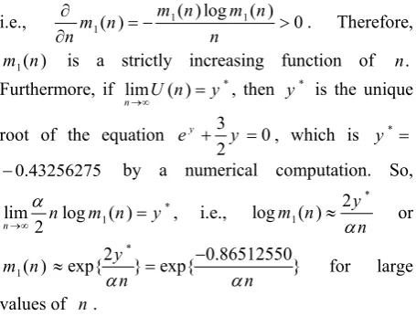
∂ . Therefore,

1( )

m n is a strictly increasing function of n. Furthermore, if _{lim ( )} *

n→∞U n =y , then *

y is the unique

root of the equation 3 0 2

y

e + y = , which is _y* ₌

0.43256275

− by a numerical computation. So,

* 1

lim log ( )

2

n n m n y

α

→∞ = , i.e.,

*

1 2

log ( )m n y n α

≈ or

1( )

m n exp{2y*} exp{ 0.86512550}

n n

α α

−

≈ = for large

values of n.

Remark 3.2 For Bernoulli ( )θ distribution, ( , )G n θ =

n

θ and equation (20) reduces to _{( )} 2

n

m m

ψ =

3 log 0.

4n m

+ = Jafari Jozani [3] showed that for Bernoulli ( )θ distribution and under the SLEL function (1), δ_π*( )X in (6) with G n m( , )=mn is a minimax

estimator of θ∈[ ,1]m if and only if * 1

m m> where * 1

m

is the unique root of the equation

*_{( )m m}2n _{3 logn m 0.}

ψ = + =

Since _ψ*_{( )m <ψ( )m for all 0<m <1, we}

conclude that * 1 1

m <m . Therefore, our result is sharper than his result. Also the work of Jafari Jozani [3] is an especial case of our result.

Table 1 summarizes a numerical solution of m1, the

root of equation (20), for different values of α and n. The first row of this table is for Bernoulli ( )θ distribution and the other rows are for the other distributions in class C1 (such as Binomial ( , )k θ ,

Negative Binomial ( , )r θ and Geeta ( , )β θ ) with suitable choices of α. From this table, we observe that

Table 1.Numericalvaluesofm1fordifferentvaluesofαandn

n

α 1 2 3 4 5 6 7 8 9 10

1 0.421 0.649 0.749 0.805 0.841 0.866 0.884 0.897 0.908 0.917 1.5 0.562 0.749 0.825 0.866 0.891 0.908 0.920 0.930 0.938 0.944 2 0.649 0.805 0.866 0.897 0.917 0.930 0.940 0.947 0.953 0.958 2.5 0.707 0.841 0.891 0.917 0.933 0.944 0.952 0.958 0.962 0.966 3 0.749 0.866 0.908 0.930 0.944 0.953 0.960 0.964 0.968 0.971

the values of m1 increase as n or α or both increases

(see Remark 3.1).

4- Conclusion

In this paper a class of discrete distributions is introduced. This class includes Binomial ( , ),k θ Negative Binomial ( , ),r θ discrete Weibull ( )θ _{and etc.} In estimation of the lower bounded parameter θ∈[ ,1]m , m>0, we find the Bayes estimator of θ under SLEL function with respect to a boundary supported prior and find a necessary and sufficient condition for which the Bayes estimator is minimax. We use the sign change method to prove the minimaxity. For a subclass of the desired discrete distributions, we find a simple necessary and sufficient condition for minimaxity and compute numerical values of m1 for different values of

α and n, for which the Bayes estimator of θ∈[ ,1]m is minimax.

Acknowledgments

The authors are grateful to the editor, two anonymous referees and Professor Ahmad Parsian of University of Tehran for making helpful comments and suggestions on an earlier version of this paper. The research of the first author was supported by the research council of Allameh Tabataba'i University. The research of the second author was supported by the research council of Islamic Azad University-Karaj Branch.

References

1. Berry C. Bayes minimax estimation of a Bernoulli p in a restricted parameter space. Commun. Statist. Theory Methods, 18: 4607-4616 (1989).

2. Brown L.D. Inadmissibility of the usual estimators of scale parameters in problems with unknown location and scale parameters. Ann. Math. Statist., 39: 29-48 (1968). 3. Jafari Jozani M. Admissible and minimax estimator of the

parameter θ in a Binomial Bin(n,θ)-distribution under squared log error loss function in a lower bounded parameter space. J. Statist. Research of Iran, 2: 139-147 (2005).

4. Jafari Jozani M., and Marchand E. Minimax estimation of constrained parametric function for discrete families of distribution. Metrika, 66: 151-160 (2007).

5. Jafari Tabrizi N., and Nematollahi N. Minimax estimation of bounded parameter of some discrete distributions under LINEX loss function. Commun. Statist. Theory Methods,

39: 2701-2710 (2010).

676 p. (2005).

7. Johnstone I., and MacGibbon B. Minimax estimation of a constrained Poisson vector. Ann. Statist., 20: 807-831 (1992).

8. Kiapour A., and Nematollahi, N. Robust Baysian prediction and estimation under squared log error loss function. Statist. Probab. Lett., 81: 1717-1724 (2011). 9. Marchand E., and Parsian A. Minimax estimation of a

bounded parameter of a discrete distribution. Statist. Probab. Lett., 76: 547-554 (2006).

10. Moors J.J.A. Estimation in truncated parameter spaces. Ph.D. Thesis, Tilburg University, Tilburg, Netherlands, 176 p. (1985).

11. Pal, N., and Ling C. Estimation of Normal scale parameter under a bounded loss function. J. Ind. Statist. Assoc., 34:

21-38 (1996).

12. Rosaco, L., De Vito, E., Caponnetto, A., Pianna, M. and Verri. Notes on the use of different loss functions.

Technical Report DISI-TR-03-07, Department of computer science, University of Genova, Italy.

13. Sajari Farsipour, N. and Zakerzadeh, H. Estimation of a gamma scale parameter under asymmetric squared log error loss function. Commun. Statist. Theory Methods, 24:

1127-1135 (2005).

14. Sajari Farsipour, N. and Zakerzadeh, H. Estimation of generalized variance under an asymmetric loss function “Squared log error”. Commun. Statist. Theory Methods,

35: 571-581 (2006).

15. van Eeden C. Restricted parameter space estimation problems admissibility and minimaxity properties. Springer, New York, 167 p. (2006).