Original Article
Comparison of auto regressive integrated moving average and artificial neural networks forecasting in mortality of breast cancer
Mohammad Moqaddasi-Amiri1, Abbas Bahrampour1*
1
Research Center for Modeling and Health, Institute for Futures Studies in Health, Department of Epidemiology and Biostatistics, School of Public Health, Kerman University of Medical Sciences, Kerman, Iran
ARTICLE INFO ABSTRACT
Available online at: http://jbe.tums.ac.ir
Background & Aim: One of the common used models in time series is auto regressive integrated
moving average (ARIMA) model. ARIMA will do modeling only linearly. Artificial neural networks (ANN) are modern methods that be used for time series forecasting. These models can identify non-linear relationships among data. The breast cancer has the most mortality of cancers among women. The aim of this study was fitting the both ARIMA and ANNs models on the breast cancer mortality and comparing the accuracy of those in parameter estimating and forecasting.
Methods & Materials: We used the mortality of breast cancer data for comparing two models. The
data are the number of deaths caused by breast cancer in 105 months in Kerman province. Each of ARIMA and ANNs models is fitted and chose the best one of each method separately, with some diagnostic criteria. Then, the performance of them is compared a minimum of mean squared error and mean absolute error.
Results: This comparison shows that the performance of ANNs models in parameter estimating and
forecasting is better than ARIMA model.
Conclusion: It seems that the breast cancer mortality has a non-linear pattern, and the ANNs
approach can be more useful and more accurate than ARIMA method. Key words:
time series, neural networks, breast cancer, auto regressive integrated moving average, mortality
Introduction1
One of the aims of modeling in statistics is forecasting based on available data and variables that could be done with methods like time series. Time series methods have many applications for forecasting in recorded events in various fields, (such as medicine, economy, and industrial) over time. In these methods, possibility model of data has been detected, and by this assumption that the model is also invariant for the future, we can forecast the data values.
* Corresponding Author: Mohammad Moqaddasi, Postal Address: Research Center for Modeling and Health, Institute for Futures Studies in Health, Department of Epidemiology & Biostatistics, School of Public Health, Kerman University of Medical Sciences, Kerman, Iran. Email: [email protected]
One of the most common models in time series is auto regressive integrated moving average (ARIMA) model. This model uses Box– Jenkins methodology in the model constructing the model (1). In this model, there are some limitations such as detecting only linearly patterns, and so the non-linear patterns will not be detected. Furthermore, the number of data must be sufficient (more than 50) until the ARIMA model can be reliable (2).
Artificial neural networks (ANNs) are modern methods that are used for time series forecasting. ANNs are data-driven that from the model based on data features (1). These models have no prior assumption and can identify non-linear relationships among data. Thus, ANNs be known as non-linear methods of time series.
The breast cancer has large mortality rate and
J Biostat Epidemiol. 2015; 1(3-4): 86-92.
the most mortality of cancers among women in the world. According to the World Health Organization statistics in 2008, the percent of mortality of breast cancer in the world, East Mediterranean region, and Iran, annually, is 13.7, 21.9, and 22, respectively (3). Hence, it is necessary that we forecast this cancer mortality with an accurate approach.
Several studies have been done in breast cancer mortality that used from the time series method for forecasting. Alvaro-Meca et al. (4) have used time series to forecast the mortality of the breast cancer in Spain. Bae et al. (5) have performed time series forecasting in cancer deaths in Korea. Yasmeen et al. (6) have forecasted age-related changes in breast cancer mortality among white and black US women by using time series analysis.
In all of the above studies, the traditional models of time series method have been used, and linear forecasting has been performed. It is possible that the breast cancer mortality pattern be non-linear. Thus, the traditional methods may not identify this pattern, and those forecasting may not accurate. The aim of this study was fitting the both traditional (ARIMA) and modern (ANNs) approaches in the modeling of the breast cancer mortality and comparing the accuracy of these models in forecasting and choosing the best one
Methods
Time series
A time series is a sequence of vectors, x(t), t = 0,1,…, where t represents elapsed time (7).
Being stationary is one of the initial conditions for using data in the time series analysis. In the stationary time series, the mean, variance, correlation, etc., are constant over time. The stationary of the data is checked by plotting data over the time and the Bartlett’s test for constant mean and variance, respectively. Differencing and variance transformations (Box-Cox) are used to make stationary a time series data in mean and variance.
There are several different traditional approaches to time series analysis that are linear such as autoregressive (AR), moving average
(MA), AR moving average (ARMA), and ARIMA. The stationary assumption for using of these models must be established. If the assumption is not true, some traditional non-linear approaches such as threshold AR and AR conditional heteroscedastic are used.
The ARIMA model
One of the most popular approaches in traditional time series models is ARIMA. This model is known as Box-Jenkins model. The general ARIMA model consists of three processes: AR, differential process for removing the trend in time series, and MA. ARIMA model notation demonstrates the order of each process with numbers. Therefore, an ARIMA(p,d,q), describes a time series with p AR order, d differential process order, and q MA order.
The values of an MA time series are a weighted average of white noise values. The values of an AR time series are a weighted average of series values. If a time series be non-stationary in mean, for estimating AR and MA process, the time series should be stationary. The differential process is used for this purpose.
ARIMA model is a combination of the listed processes. The mathematical form of this model is as follow:
y = a y + a y + ⋯ + a y + ε − β ε −
β ε − ⋯ − β ε
(3)
where yt is the actual value; and εt is the random error at time period t; αi(i = 1, 2, …, p) and
βj(j = 0, 1, 2,…, q) are model parameters. The p and q are the orders of model.
Based on Box and Jenkins methodology, there are three steps to build an ARIMA model including model identification, parameter estimation, and diagnostic checking. These steps will be continued and repeated to achieve the appropriate model. In the identification step, the orders of the ARIMA model can be identified. To determine the order of MA and the order of AR, the autocorrelation function (ACF) and the partial ACF (PACF) will be used, respectively. It is possible to identify one or more potential models for the data. In this step, the stationary of the time series must be checked, and the data be
transformed if necessary.
In the second step, the model parameters and an overall measure of errors like mean squared errors (MSE) are be estimated, In this step several models may be fitted. The best model is selected with the minimum of them.
The third step is the diagnostic checking of the model adequacy. Some diagnostic statistics and plot of the residuals such as ACF and PACF plots of residuals, can be used for checking the goodness of fit of the model. If the model is not adequate, another model should be selected.
ANN
The ANN is another method that used to fit the non-linear time series model. There are limitations in the use of traditional non-linear time series, but the ANNs have no prior assumptions and can discover the non-linearity patterns, even in small data sets. Because of parallel processing of the data, “ANNs can approximate a large class of functions with a high degree of accuracy” (1).
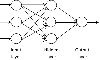
There are many ANN models, but “the most influential models are the multi-layer perceptrons (MLP)” (8). The MLP networks have large applications in forecasting. The MLP is formed of several layers of nodes. The first layer is an input layer where information or data enter into the network. The last layer is an output layer where the outcome of the model obtained. Between these two layers, there are one or more layers that called hidden layers. The nodes in these layers are fully interconnected by arcs. We can divide the MLP models to feed forward and recurrent models. In the feed forward, the direction of processing’s arcs is from input to output nodes without returning to the back. The recurrent models have arcs that return back from the output or hidden nodes to input nodes. We used a feed forward MLP network with one hidden layer in our study. Each arc has a weight that estimated by a process called training.
Training
For using of an ANN in any desired task, the network must be trained first. In this process, the parameters of the network that are the weight of
the arcs be estimated. By training process, an ANN can find out complex non-linear patterns and estimates the best weights. ANNs in training be divided into supervised and unsupervised. In the supervised training, both input and output vectors in the network are defined, but the unsupervised training has only input vector. The MLP training is a supervised approach.
The data usually are divided into a training set and a test set. The training set is a sample of the data that be used for estimating the weights. The test set can be a sample of the data or out of it, and used for measuring the generalization ability of the network. Usually, the test set is selected a sample of the data. In this case, the size of the test set is different between 10% and 30% of the data. The best one is chosen with the minimum of MSE by testing the network, after training it.
The network architecture
In designing the MLP network, we must determine the number of nodes in each layer. The selection of these parameters has no defined algorithm and depends on the type of research. In some methods like regression, the number of input nodes is considered equal to the number of independent variables. In time series data, we have a sequence of observations during the time that make difficult the selection of the number of input nodes. The number of hidden nodes in its layer has no specific selection algorithm. Based on forecasting horizon, the output nodes can be one or more. In one-step-ahead forecasting, there is one output node and in multi-step-ahead the number of output nodes can be one or more. We used the multi-step-ahead forecasting with one output node in the output layer. We tested various numbers of input and hidden nodes, and then selected the best of them. An ANN (i,h,o), describes a network with i input nodes, h hidden nodes, and o output nodes (Figure 1).
Figure 1. A typical atypical feed forward neural network with one hidden layer
Activation function
Activation or transfer function determines the relationship of inputs and outputs of a node by introducing a degree of non-linearity. There are some activation functions such as sigmoid (logistic), hyperbolic tangent (tanh), tansig, and linear. Different functions were tested in our MLP network, and then we selected the best one.
ANN method to time series modeling
For fitting a single hidden layer feed forward network for time series modeling the following formulation is used:
q p
t 0 j 0j ij t 1 t
j=1 i=1
y =α + αgβ + β y− +ε
∑
∑
(4)
where αj and βij are the model parameters or arcs weights. p is the number of input nodes and q is the number of hidden nodes. This model has one output node in the output layer. After fitting the model, the network performs the following function mapping:
(
)
t t 1 t 2 t p t
y =f y , y− − ,K, y− , w +ε
(5)
where (yt−1, yt−2,…, yt−p) are the past observations; yt is the future value; w is a vector of parameters; and f is a function determined by the network. “Thus, the neural network is equivalent to a non-linear AR model” (1).
We fitted the ARIMA models and chose the best one with the minimum of MSE, Akaiki information criteria (AIC), Bayesian information criteria (BIC), and corrected AIC (AICc). Then, we built the networks with different numbers of input and hidden nodes, different activation functions in hidden and output layers, and different sizes of training and testing sets. The best network was selected with the minimum of MSE and mean absolute error (MAE).
All these analyze were performed in MINITAB16 software also forecast (10) and AMORE (11) packages in R software.
Data set
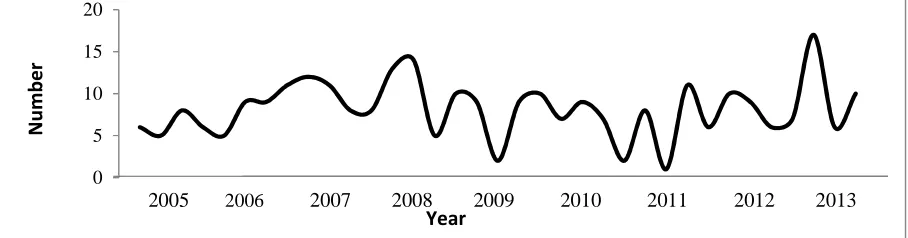
The data are the number of deaths caused by breast cancer in 105 months in Kerman province, collected in the cancer registry of Kerman University of Medical Sciences, during 2005-2013.
Results
Time series results
Non-stationary in variance was concluded from the Bartlett test (P = 0.04). The Box-Cox transformation (λ = 0.28) used to make the data stationary in variance. The time series plot shows that the mean of the data approximately is constant over the time, but we fitted ARIMA models with and without differencing on data for choosing the best one (Figure 2).
Input layer
Hidden layer
The ACF and PACF of the transformed data were plotted to detect the order of potential ARIMA models. Some ARIMA models were diagnosed, so we fitted these models and obtained the overall measures of accuracy (Table 1).
According to the table 1, the best ARIMA model based on MSE was ARIMA(1,0,1) or ARMA(1,1) and based on AIC, AICc, and BIC was ARIMA(0,1,1). We used these models for comparing with the best network of ANNs method. The goodness of fit of these models checked. The ACF and PACF of residuals had no problem, and there was the normality of residuals. The fitted models are as follow:
ARIMA(0,1,1): yt= 0.9112 εt−1 (8)
ARMA(1,1): yt = 1.46−0.46 yt−1−0.57 εt−1 (9)
Neural networks results
As mentioned earlier in the method section, we tested several ANNs with various numbers of input and hidden nodes and different activation functions for the hidden and output layer. We applied sigmoid, tansig, and linear functions as the hidden and output activation functions.
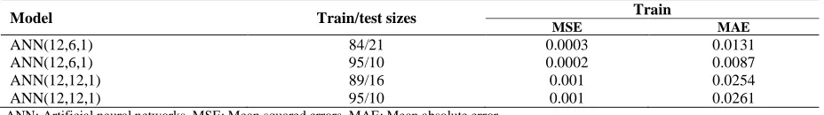
Table 2 shows best models of ANNs with various sizes of training and testing set. Models with sigmoid and linear function as hidden and
output activation functions, respectively, were the best. Networks with different number of input and hidden nodes were applied with these two functions. According to the MSE and MAE, the networks with 12 nodes in inputs and 6 nodes in hidden layers are more accurate than others. We chose the ANN(12,6,1) network with 84 and 95 months in training set as the best models of ANNs. The accuracy of these models in estimating the parameters (training) has no large difference in MSE and MAE (Table 2).
To assess the performance of forecasting we forecasted 21 and 10 last observations of data by the first two networks of table 2, respectively, and then compared with forecasting of the best ARIMA model. The results are presented in table 3.
Discussion
In this research, we compared the accuracy of ANN and ARIMA models to forecast mortality of breast cancer. As shown in the results, the ANN model forecasts were more accurate than ARIMA model. By this conclusion, we propose that in future studies on breast cancer mortality, be used from ANNs for forecasting. Among ARIMA models, ARMA(1,1) has better performance in forecasting than other models.
Figure 2. The plot of seasonal time series for the breast cancer mortality
Table 1. Best ARIMA models of breast cancer mortality
Model MSE AIC AICc BIC
ARIMA(1,0,1) 0.5302 239.38 239.78 250
ARIMA(0,1,1) 0.5522 239.15 239.27 244.14
ARIMA(1,1,1) 0.5516 241.07 241.31 249.01
ARIMA(2,1,1) 0.5416 241.11 241.51 251.68
ARIMA(3,1,1) 0.5415 243.09 243.7 256.31
ARIMA: Auto regressive integrated moving average, MSE: Mean squared errors AIC: Akaiki information criteria, BIC: Bayesian information criteria, AICc: Corrected Akaiki information criteria
0 5 10 15 20
2005 2006 2007 2008 2009 2010 2011 2012 2013 Year
N
u
m
b
e
Table 2. Best networks of breast cancer mortality
Model Train/test sizes Train
MSE MAE
ANN(12,6,1) 84/21 0.0003 0.0131
ANN(12,6,1) 95/10 0.0002 0.0087
ANN(12,12,1) 89/16 0.001 0.0254
ANN(12,12,1) 95/10 0.001 0.0261
ANN: Artificial neural networks, MSE: Mean squared errors, MAE: Mean absolute error
Table 3. Comparison between the performance of the ARIMA and ANNs in forecasting
Model 10 points ahead 21 points ahead
MSE MAE MSE MAE
ARIMA(1, 0, 1) 0.489 0.587 0.475 0.540
ARIMA(0, 1, 1) 0.601 0.630 0.597 0.616
ANN(12, 6, 1) 0.030 0.014 0.0004 0.013
ARIMA: Auto regressive integrated moving average, ANN: Artificial neural networks, MSE: Mean squared errors, MAE: Mean absolute error
According to the table 2, the accuracy of ANN models in estimating the parameters (training) has no large difference in MSE and MAE, but they were more accurate than ARIMA models in parameter estimating.
The performance of ANNs models in parameter estimating and forecasting is better than ARIMA model, and there are large differences in MAE and MSE between two methods.
This conclusion is as same as many researches in various fields that ANN methods had better performance than traditional methods. Lachtermacher and Fuller that investigated on 4 stationary river flow and 4 non-stationary electricity load data and concluded that ANNS have a slightly better overall performance than ARIMA in stationary data and much better in non-stationary (12). Kohzadi et al. compared these methods for US monthly live cattle and wheat cash prices and resulted that the neural network forecasts were considerably more accurate than those of the traditional ARIMA models (13). Caire et al. concluded that ANNs are hardly better than ARIMA for the one-step-ahead forecast in one electric consumption data (14). Furthermore, Kang (15), Sharda and Patil (16), Portugal and de Pós-Graduação (17), Chakraborty et al. (18) show that ANNs were more accurate than traditional ARIMA models.
The ARIMA models have larger MSE and MAE in parameter estimating and forecasting than the best ANNs model. Thus, it seems that the breast cancer mortality has a non-linear pattern, and the ANNs approach can be more useful and more accurate than ARIMA method.
Acknowledgments
In this way, the health department based cancer registry in Kerman University is appreciated. Corporation of vice chancellor of research of Kerman University of Medical Sciences for financial support of this project is acknowledged. This project is part of Mohammad Moqaddasi Amiri Thesis for Master of Science in Biostatistics.
References
1. Zhang GP. Time series forecasting using a hybrid ARIMA and neural network model. Neurocomputing 2003; 50: 159-75.
2. Imhoff M, Bauer M, Gather U, Löhlein D. Time series analysis in intensive care medicine. Applied Cardiopulmonary Pathophysiology 1997; 6(263): 81.
3. International Agency for Research on Cancer. The globocan project [Online]. [cited 2012]; Available from: URL:
http://globocan.iarc.fr/Default.aspx
4. Alvaro-Meca A, Debon A, Gil PR, Gil de Miguel A. Breast cancer mortality in Spain: has it really declined for all age groups? Public Health 2012; 126(10): 891-5.
5. Bae JM, Jung K, Won YJ. Estimation of cancer deaths in Korea for the upcoming years. J Korean Med Sci 2002; 17(5): 611-5. 6. Yasmeen F, Hyndman RJ, Erbas B. Forecasting age-related changes in breast cancer mortality among white and black US women: a functional data approach. Cancer
Epidemiol 2010; 34(5): 542-9.
7. Frank RJ, Davey N, Hunt SP. Time Series Prediction and Neural Networks. Journal of Intelligent and Robotic Systems 2001; 31(1-3): 91-103.
8. Zhang G, Patuwo BE, Hu MY. Forecasting with artificial neural networks: The state of the art. International Journal of Forecasting 1998; 14(1): 35-62.
9. Kaastr I, Boyd M. Designing a neural network for forecasting financial and economic time series. Neurocomputing 1996; 10(3): 215-36.
10. Hyndman RJ. Forecast package for R [Online]. [cited 2014 May 8]; Available from: URL:
http://robjhyndman.com/software/forecast/ 11. Limas MC, Ordieres Mere JB, Marcos AG,
Martinez FJ, de Pison Ascacibar F, Espinoza AV, et al. AMORE: A MORE flexible neural network package [Online]. [cited 2014 Apr 14]; Available from: URL:
http://cran.r-project.org/web/packages/AMORE/index.html 12. Lachtermacher G, Fuller JD. Back propagation in time-series forecasting.
Journal of Forecasting 1995; 14(4): 381-93. 13. Kohzadi N, Boyd MS, Kermanshahi B,
Kaastra I. A comparison of artificial neural network and time series models for
forecasting commodity prices.
Neurocomputing 1996; 10(2): 169-81. 14. Caire P, de France E, Hatabian G, Muller C.
Progress in forecasting by neural networks. Baltimore, MD: Neural Networks, IJCNN, International Joint Conference on; 1992. 15. Kang SY. An investigation of the use of
feedforward neural networks for forecasting [Thesis]. Kent, OH: Kent State University 1992.
16. Sharda R, Patil RB. Connectionist approach to time series prediction: an empirical test. Journal of Intelligent Manufacturing 1992; 3(5): 317-23.
17. Portugal MS, de Pós-Graduação C. Neural networks versus time series methods: a forecasting exercise. Revista Brasileira de Economia 1995; 49(4): 611-29.