Well-posedness of an epidemiological problem described by an evolution PDE

(1)

E. Canc`es, S. Faure, B. Graille, Editors

WELL-POSEDNESS OF AN EPIDEMIOLOGICAL PROBLEM DESCRIBED BY

AN EVOLUTION PDE

A. Perasso

1,2

and B. Laroche

2

Abstract. This paper investigates the well-posedness for a non linear transport equation system that models the spread of prion diseases in a managed flock. Existence and uniqueness of solutions are proved with the use of semigroup theory in the case of a Lipschitz perturbation and presence of boundary conditions. Finally, the characteristics of the transport part of the equations allow us to give an implicit expression of the solution.

Résumé. Dans ce papier, nous établissons le caractère bien posé d’un problème de transport non linéaire modélisant la propagation d’une maladie à prion dans un troupeau expérimental. Nous prou-vons existence et unicité de la solution du problème à l’aide de la théorie des semigroupes, avec présence de conditions de bord et une partie non linéaire localement lipschitzienne. Nous donnons pour conclure une expression implicite de la solution utilisant les caractéristiques des équations de transport.

Introduction

The prion pathologies are characterized by a long incubation period, relative to lifespan, during which the disease cannot be detected. At the end of the incubation period, animals develop distinctive clinical signs which are rapidly followed by death. The confounding effects of incubation, natural mortality and the changing force of infection make direct analysis difficult. A mathematical model of the within-population transmission dynamics provides a flexible tool for combining epidemiological and demographic phenomenon.

In this paper, we study the well-posedness of a problem of propagation of a prion disease in a managed popula-tion. The model we consider takes into account the population dynamics as well as the spread of the outbreak. Owing to the long incubation period, population demography and management must be included in the model. The mathematical model is therefore formulated in terms of population densities structured according to disease status (Susceptible and Infected), to age and to infection load for infected animals. This leads to a nonlinear integro partial differential dynamical system of transport type.

The first part of the paper is dedicated to the description of the model. In a second part, we establish the well-posedness of the problem. In order to reach that goal we start with the study of the linear part of the prob-lem with the use of semigroup theory. Then we conclude for our initial probprob-lem adapting arguments developed in [10].

1 _{Laboratoire de Math´ematiques, Bˆ}_{atiment 425, Universit´e Paris-Sud XI, F-91405 Orsay Cedex, France.}

2 _{Laboratoire des signaux et syst`emes (L2S) Sup´elec - 3 rue Joliot-Curie 91192 Gif-sur-Yvette cedex, France.}

c

EDP Sciences, SMAI 2008

(2)

1. Description of the model

To take into account human management of the population, we assume that ageabelongs to a finite interval [0, A], animals reaching ageAbeing systematically culled because they are considered as too old. The population of infected animals is also structured according to the infection load variable θ that lies in interval [0,1]. The densities of Susceptible and Infected are denoted asS(t, a) andI(t, a, θ), and the number of infected animals at timet is denoted

K(I)(t) :=

Z A

0

Z 1

0

I(t, a, θ)dθda. (1)

The model we use is a simplified version inspired from an epidemic model in [12]. It is a modified version of the classical Kermack-McKendrickSIepidemiological PDE model [6–8] or [9]. The underlying assumptions are homogeneous mixing between all the individuals and a constant probability transmission per contact, β > 0, giving a net rate of infection of β S K(I). This is known as themass action assumption, and comes from a classical microscopic modeling by birth-death processes [5].

Incubation time heterogeneity is modeled through the infection load variable θ. It is assumed that θgrows exponentially with time with an infection load velocityc > 0. Infected animals with infection load less than 1 cannot be detected, although they are infectious. An infection load equal to 1 corresponds to the onset of clinical signs and immediate death, either caused by the disease or by culling.

When infection occurs, an animal gets an initial infection load θ0 ∈]0,1[, so that the incubation time τ is

given by

τ =−1

c lnθ0.

Variable incubation time in the infected population is therefore represented by a probability density function (pdf) Θ of the initial infection load that satisfies

Θ∈ A(0,1), Θ(0) = Θ(1) = 0,

whereA(0,1) is the set of real-analytic functions on ]0,1[ continuous on [0,1]. The role of the pdf Θ is to attribute an initial infection load, and therefore an incubation time, to susceptible animals when they get infected. Such an approach is related to the so-called ”size-structured models” encountered in cellular population dynamics (see [1] for a review). An alternative option would be to structure the infected population according to the age of infection like in [2, 3]. Whatever the parametrization, it leads to a distributed delay structure.

DensitiesS andI satisfy the following transport equations for (t, a, θ)∈[0,+∞[×[0, A]×[0,1] :

∂S ∂t +

∂S

∂a =−µS−βSK(I), (Evol1)

∂I ∂t +

∂I ∂a+

∂(c θ I)

∂θ =−µI+βΘSK(I). (Evol2)

Parameterµ >0 in the model is the basic disease free mortality rate. Infected animals have a strictly positive infected load and we assume in this model that there is no vertical (in utero) transmission. Consequently we associate to the equations (Evol1)–(Evol2) the following boundary conditions, wheret _7→n(t) represents the birth function :

(

S(t,0) =n(t),

I(t,0, θ) = 0, I(t, a,0) = 0, for (t, a, θ)∈[0,+∞[×[0, A]×[0,1]. (Bc)

The initial conditions are given by

(

S(0, a) =S0(a),

I(0, a, θ) =I0(a, θ),

(3)

In the following, we will denote (P) the problem

(P)

(Evol1)−(Evol2),

(Bc)−(Ic).

2. Well-posedness of the problem

The Problem (P) is a nonlinear Cauchy problem with a boundary condition, that can be viewed as a perturbation of a linear problem. Consequently, we prove the existence and uniqueness of solutions taking into account a non zero boundary condition. First, we use the ideas of [4] in order to delete the boundary condition and to reduce our problem to a Cauchy problem. Then we adapt the arguments of [10] to prove existence and uniqueness of mild solutions of this Cauchy problem in the positive cone of a Banach space of real valued functions. Finally we deduce the existence and uniqueness of mild solutions for our initial problem (P) and conclude about the well-posedness.

2.1. Lifting of boundary conditions

We perform a change of variables in order to transform the boundary condition (Bc) into a null condition. For a Banach space (E,k·kE) of real valued functions and any setF ⊂E,F+shall denote the subset of positive functions of F. We also setX = L2₍₀_{, A}₎_×_L2 ₍₀_{, A}₎_×₍₀_,₁₎

and we denote k · kS, and k · kI, the norm in L2(0, A), respectively in L2 (0, A)×(0,1)

, andk · kX :=k · kS +k · kI the product norm on X. We suppose that (S0, I0)∈L2(0, A)+×L2 (0, A)×(0,1)

+

andn_∈Cpw([0,+∞[)+, where Cpw([0,+∞[) denotes the set of

piecewise continuous functions onR+.

We considerB: [0,+∞[→ L Cpw(0,+∞),L2(0, A)defined for allg∈Cpw(0,+∞) by

(B(t)g)(a) :=

(

g(0)e−µt _for_a_∈_[0_{, A}_]_{, a}_≥_t,

g(t−a)e−µa _for_a_∈_[0_{, A}_]_{, a}_≤_t,

and the new system

∂S˜

∂t =−

∂S˜

∂a−µS˜−β( ˜S+B(t)n)K( ˜I), ( ˜Evol1)

∂I˜ ∂t =−

∂I˜ ∂a−

∂(c θI˜)

∂θ −µI˜+βΘ ( ˜S+B(t)n)K( ˜I), ( ˜Evol2)

with boundary condition

( _˜

S(t,0) = 0,

˜

I(t,0, θ) = ˜I(t, a,0) = 0, ∀(t, a, θ)∈[0, T]×[0, A]×[0,1], ( ˜Bc)

and initial condition

( _˜

S(0, a) = ˜S0(a) =S0(a)−n(0),

˜

I(0, a, θ) = ˜I0(a, θ) =I0(a, θ),

∀(a, θ)∈[0, A]×[0,1]. ( ˜Ic)

Remark 2.1. For allg_∈Cpw(0,+∞),B(t)g satisfies the following transport equation

∂B(t)g

∂t +

∂B(t)g

(4)

and fort >0,B(t)g(0) =g(t).

Consequently, the transformationS_7→S˜:=S₋B(t)nimplies that ˜Ssatisfies equations ( ˜Evol1)-( ˜Evol2) with conditions ( ˜Bc)-( ˜Ic) iffS satisfies Problem (P).

Let ΦS and ΦI be the differential operators defined by

ΦS :D(ΦS)→L2(0, A), ΦI :D(ΦI)→L2 (0, A)×(0,1), (2)

f 7→ −f0−µ f, f 7→ −∂af−∂θf−(µ+c)f, (3)

whereD(ΦS) andD(ΦI) are the following sets :

D(ΦS) :={f ∈C1[0, A], f(0) = 0},

D(ΦI) :={f ∈C1([0, A]×[0,1]), f(·,0) =f(0,·) = 0}.

Setting ˜u(t) :=S˜(t,·),I˜(t,·), ˜u0:= ( ˜S0,I˜0), Φ :D(Φ)→X where D(Φ) :=D(ΦS)×D(ΦI)⊂X is given by

Φ :=

ΦS 0 0 ΦI

, (4)

and

˜

P : [0,+∞[×X_→X, (t,(˜uS,˜uI))7→

_˜

PS ˜

PI

:=

−β(˜uS+B(t)n)K(˜uI)

βΘ (˜uS+B(t)n)K(˜uI)

,

well-posedness of equations ( ˜Evol1)–( ˜Evol2) with initial condition ( ˜I c) is equivalent to well-posedness of the following problem

( ˜P)

( _d

dtu˜(t) = Φ˜u(t) + ˜P(t,u˜(t)), ˜

u(0) = ˜u0.

2.2. The linear problem

This section is devoted to the definition of the semigroups generated by the differential operator Φ for the linear problem.

Proposition 2.2. ΦS and ΦI are infinitesimal generators of two strongly continuous positive semigroups of

bounded linear operators, TS: [0,+∞[→ L(L2(0, A))andTI : [0,+∞[→ L(L2 (0, A)×(0,1)

), defined by

(TS(t)f)(a) :=

(

f(a₋t)e−µt _for _a_≥_t,

0 for a_≤t, for allf ∈L

2₍₀_{, A}₎_,

and

(TI(t)f)(a, θ) :=

(

f(a−t, θe−ct₎_e−(µ+c)t _for _a_≥_t,

0 for a_≤t, for allf ∈L

2 ₍₀_{, A}₎

×(0,1) .

We have moreover the following estimation :

sup(kTS(t)k, kTI(t)k)≤e−µt ∀t≥0. (5)

Proof. We can easily check that (TS(t))t≥0 and (TI(t))t≥0 are semigroups of bounded strongly continuous

operators.

In order to prove that ΦI, respectively ΦS, is the infinitesimal generator ofTI, respectivelyTS, we prove that

lim t→0

TI(t)f −f

t −ΦIf

(5)

Forf _∈D(ΦI) and fort >0,

TI(t)f −f

t −ΦIf

2 I

≤(A₋t) sup

(a,θ)∈[t,A]×[0,1]

(TI(t)f)(a, θ)−f(a, θ)

t −ΦIf(a, θ)

2 + Z t 0 Z 1 0

f(a, θ)

t −ΦIf(a, θ) 2 dθ da. (6)

The last term in the right hand side of (6) can be bounded as follows :

Z t 0 Z 1 0

f(a, θ)

t −ΦIf(a, θ)

2

dθ da≤2

Z t 0 Z 1 0

f(a, θ)

a 2 dθ da

+2t sup

(a,θ)∈[0,A]×[0,1]|

ΦIf(a, θ)|2.

(7)

Sincef _∈D(ΦI), using the Lebesgue dominated convergence theorem in (7) we have

lim t→0 Z t 0 Z 1 0

f(a, θ)

t −ΦIf(a, θ)

2

dθ da= 0. (8)

Letf _∈D(ΦI) and the functionGdefined on the subsetEI :={(t, a, θ)∈[0,+∞[×[0, A]×[0,1], a≥t}by :

G(t, a, θ) :=



 

 

f(a−t, θ e−ct₎_e−(µ+c)t₋_f₍_{a, θ}₎

t t6= 0,

ΦIf(a, θ) t= 0.

We can see in Proposition 3.1 of appendix, that G is continuous on EI and then is uniformly continuous. Consequently,

lim

t→0₍_a,θ_)∈[sup_t,A_]×[0_,_1]

(TI(t)f)(a, θ)−f(a, θ)

t −ΦIf(a, θ)

= 0, (9)

and we conclude using the limits in (8) and (9) reported in (6). Similar considerations prove that ΦS is the infinitesimal generator ofTS.

Estimation (5) as well as the positivity ofTS andTI are easily derived from their expressions.

We now define the concept of mild solution, and give the two main results of the paper related to well-posedness.

Definition 2.3. A mild solution of Problem ( ˜P) is a function ˜u_∈C([0,+∞[, X) that satisfies ˜

u(t) =T(t)˜u0+

Z t

0

T(t−s) ˜P(s,u˜(s))ds ∀t∈[0, T]. (10)

The following result holds,

Theorem 2.4. Suppose thatS0∈L2(0, A)+,I0∈L2 (0, A)×(0,1) +

andn∈Cpw(0,+∞)+. Then the problem

( ˜P)has a unique mild solutionu˜:= ( ˜S,I˜)such thatI˜(t)≥0andS˜(t) +B(t)n_≥0for allt_≥0.

Consequently,

Corollary 2.5. If n∈Cpw(0,+∞)+, then for allu0:= (S0, I0)∈L2(0, A)+×L2 (0, A)×(0,1) +

the Problem

(P)has a unique mild solutionu:= (S, I)∈C([0,+∞[, X)in the following sense :

S(t, a) =







(TS(t)S0)(a) +R₀t TS(t−s)PS(u(s))(a)ds for a≥t,

(B(t)n)(a) +Rt

0 TS(t−s)PS(u(s))

(a)ds for a≤t,

(6)

and

I(t, a, θ) = (TI(t)I0)(a, θ) +

Z t

0

TI(t−s)PI(u(s))

(a, θ)ds, (12)

whereS(t) andI(t)are positive functions for allt_∈[0,+∞[.

Moreover, for all T > 0 and all u0, v0 ∈ L2(0, A)+×L2 (0, A)×(0,1) +

, there exists K > 0 such that the associated mild solutionsu, v satisfy

ku(t)−v(t)kX≤Kku0−v0kX ∀t∈[0, T]. (13)

The next section is devoted to the proof of these main results. In order to prove them, we start with the study of the non-linear semi-group.

2.3. The nonlinear problem

A consequence of Proposition 2.2 is that for all ˜u0∈D(ΦS)×D(ΦI), the linear problem associated to ( ˜P) has a unique classical solution given by ˜u(t) =T(t) ˜u0 fort≥0. For ˜u0∈X, we now look for a mild solution

of ( ˜P) as the sum of the solution of the linear problem and a term accounting for the perturbation ˜P. To this end, we need a local control of the perturbation ˜P. This is done in the following proposition.

Proposition 2.6. The perturbationP˜is a locally Lipschitz function inu= (uS, uI), uniformly inton segments

of R+ : for allr >0and all T >0there existsm(r, T)>0such that

kP˜(t, u1)−P˜(t, u2)kX≤m(r, T)ku1−u2kX ∀u1, u2∈BX(0, r), ∀t∈[0, T].

Moreover,r_7→m(r, T)is a growing continuous function.

Proof. LetT, r >0 andu1:= (uS1, uI1),u2:= (uS2, uI2) such that (u1, u2)∈(BX(0, r))

2_{. Then for all}_t_∈_[0_{, T}_]

we have

kP˜(t, u1)−P˜(t, u2)kX =kβ(uS2+B(t)(n))K(uI2)−β(uS1+B(t)(n))K(uI1)kS +kβΘ (uS1+B(t)n)K(uI1)−βΘ (uS2+B(t)n)K(uI2)kI.

(14)

Using expression ofK(I) and Cauchy-Schwarz inequality we have

kβ(uS2+B(t)n)K(uI2)−β(uS1+B(t)n)K(uI1)k

2

S ≤2β2k(uS2+B(t)n)K(uI1−uI2)k

2 S

+ 2β2k(uS1−uS2)K(uI1)k

2 S

≤2β2A kuS2+B(t)nk

2

SkuI1−uI2k

2 I

+kuI1k

2

IkuS1−uS2k

2 S

.

Since for allt∈[0, T]

kB(t)nk2S =

Z min(t,A)

0 |

n(t−a)|2e−2µa da+

Z A

min(t,A) |

n(0)|2e−2µt da≤ knk2L2₍₀_,T₎+A|n(0)|

2

,

we obtain for allt∈[0, T] the following upper bounds

2 S ≤

2β2A 

 r+ sup

t∈[0,T]k

B(t)nkS

!2

kuI1−uI2k

2

I +r2k(S1−S2)k2S

!

(7)

and settingc(r, T) := 2β2_A₍_r_{+ sup} t∈[0,T]k

B(t)n_k2_S), we deduce

2

S ≤c(r, T)ku1−u2k2X.

We also have for allt_∈[0, T]

kβΘ (uS1+B(t)n)K(uI1)−βΘ (uS2+B(t)n)K(uI2)k

2

I ≤c(r, T)kΘk2∞ku1−u2k 2 X.

Using (14) we can conclude, settingm(r, T) :=p

c(r, T)(1 +kΘk2 ∞), that

kP˜(t, u1)−P˜(t, u2)kX ≤m(r, T)ku1−u2kX.

We can easily check thatr7→m(r, T) is a growing function using definitions ofc(r, T) andm(r, T).

We now prove the Theorem 2.4 using a fixed point method adapting the proof of [11]. Consider T > 0,

r:= 2(ku0kX+knkL2₍₀

,T)+ supt∈[0,T]kB(t)nkS) andδ >0 such that

δ <min

(

T, 1

2m(r, T),

1

β√A(kn_k2

L2₍₀_,T₎+kS0k2_S) 1

2 +m(r, T)

)

.

We define the mappingF :C([0, δ], X)→C([0, δ], X) by

Fu˜(t) :=

FSu˜(t)

FIu˜(t)

:= g(t)−B(t)n

TI(t) ˜I0+

Rt

0 TI(t−s) ˜PI(s,u˜(s))ds

!

,

where

g(t) :a_7→ 





S0(a−t)e−(µt+β

Rt

0K( ˜I)(s)ds) ifa≥t,

n(t₋a)e−(µa+βRtt−aK( ˜I)(s)ds) ifa≤t.

(15)

Lemma 2.7. The mapping F preserves the closed subset_F defined by

F:=

(

˜

u:= ( ˜S,I˜)∈C([0, δ], X), sup t∈[0,δ]k

˜

u(t)kX≤r, S˜(t) +B(t)n≥0andI˜(t)≥0

)

.

Moreover F is a contraction mapping on F.

Proof. Let ˜u_{∈ F}. SincekTI(t)k ≤1,

kFu˜(t)kX≤ kS0kS+knkL2₍₀_,T₎+ sup t∈[0,T]k

B(t)n_kS+kI˜0kI+

Z t

0 k

TI(t−s)k

kP˜I(s,u˜(s))−P˜I(s,0)kI+kP˜I(s,0)kI

ds

≤ ku0kX+knkL2₍₀_,T₎+ sup t∈[0,T]k

B(t)n_kS+

Z t

0

(r m(r, T) + 0) ds

≤ ku0kX+knkL2₍₀

,T)+ sup t∈[0,T]k

B(t)nkS+t r m(r, T),

and using definition ofδandr

(8)

Moreover, we can easily check that FSu˜(t) +B(t)n ≥0, and then ˜PI(s,u˜(s))≥ 0. Since ˜I0 ≥0 and TI is a positive semigroup, we can conclude FIu˜(t)≥0 andF preservesF. Now, let us prove thatF is a contraction mapping. We can see in Proposition 3.2 in appendix that for ˜u1,u˜2∈ F,

kFSu˜1(t)−FSu˜2(t)kS≤β √

A t(kS0k2S+knk 2 L2₍₀

,T))

1

2 sup

t∈[0,δ]k

˜

u1(t)−u˜2(t)kX ∀t∈[0, δ]. (16)

Furthermore,

kFIu˜1(t)−FIu˜2(t)kI ≤

Z t

0 k

˜

PI(s,u˜1(s))−P˜I(s,u˜2(s))kI ds

≤m(r, T)t sup t∈[0,δ]k

˜

u1(t)−u˜2(t)kX ∀t∈[0, δ]. (17)

With (16) and (17) we have for allt_∈[0, δ]

sup t∈[0,δ]k

Fu˜1(t)−Fu˜2(t)kX≤

m(r, T) +β√A(kS0k2S+knk2L2₍₀_,T₎) 1 2

δ sup

t∈[0,δ]k

˜

u1(t)−u˜2(t)kX,

which guarantees that F is a contraction mapping onF.

Consequently to lemma 2.7,F has a unique fixed point ˜u= ( ˜S,I˜) inF. We now prove that this solution can be extended to [0, T].

Let us suppose that ˜u is defined on some interval [0, τ], 0 < τ < T. As in Proposition 3.3 of appendix we consider ˜uτ(t) = ( ˜Sτ(t),I˜τ(t)) the unique solution on [τ, τ+δτ] of

˜

uτ(t) =

gτ(t)−B(t)n

TI(t−τ) ˜I(τ) +

Rt

τ TI(t−s) ˜PI(s,u˜τ(s))ds

!

, (18)

with

gτ(t) :a7→







g(τ, a−(t−τ)e−(µ(t−τ)+β

Rt

τK( ˜Iτ)(s)ds) _if

a≥t−τ ,

n(t₋a)e−(µa+βRtt₋aK( ˜Iτ)(s)ds)

ifa_≤t₋τ ,

δτ<min

(

T −τ, 1

2m(rτ_{, T}₎,

1

β√A(knk2

L2₍₀_,T₎+kS˜(τ) +B(τ)nk2_S) 1

2 +m(rτ, T)

)

,

and

rτ _{:= 2 (}_k_S

0kS+knkL2₍₀_,T₎+kI˜(τ)kI + sup t∈[0,T]k

B(t)n_kS). (19)

We also prove in Proposition 3.3 of appendix that the function ˜ucan be extended to [0, τ+δτ_{] defining ˜}_u_{:= ˜}_u τ on [τ, τ+δτ]. Clearly ˜uis in C([0, τ+δτ], X).

LetJ ⊂[0, T] be the maximal interval of existence of the solution ˜u, and let us denotetmax:= supJ. We can check that there exists a constantCT >0 independent oftmaxsuch that for allt∈J

ku˜(t)kX ≤CT. (20)

Indeed, using expression ofgτ and (18), we can easily check that

˜

S(t, a) =g(t, a)−(B(t)n)(a) ∀(t, a)∈J×[0, A], (21)

and then for allt∈J

kS˜(t)kS≤ kS0kS+knkL2₍₀

,T)+ sup t∈[0,T]k

(9)

For ˜I we have

kI˜(t)kI ≤ kI˜0kI+

Z t

0 k

TI(t−s)k kP˜(s,u˜(s))kI ds.

Using the following estimations

kP˜I(t,u˜(t))kI ≤βkΘkL2₍₀

,1)kg(t)kS √

AkI˜(t)kI

≤β√AkΘkL2₍₀_,₁₎(kS₀kS+knk_L2₍₀_,T₎)kI˜(t)kI,

we can deduce, denotingc:=β√A_kΘkL2₍₀_,₁₎(kS₀kS+knk_L2₍₀_,T₎), that for allt∈J

kI˜(t)kI ≤ kI˜0kI+c

Z t

0 k

˜

IkI ds.

By Gronwall’s inequality we finally obtain

kI˜(t)kI ≤ kI˜0kIect ∀t∈J. (23)

Consequently to (22) and (23), we deduce (20) withCT =kI˜0kIecT+kS0kS+knkL2₍₀

,T)+ supt∈[0,T]kB(t)nkS.

This uniform bound on the solutions guarantees the existence of a global-in-time solution on [0, T], as stated in [10] or [11]. Moreover, clearly ˜u∈C([0, T], X) and satisfies ˜I(t)≥0 and ˜S(t) +B(t)n≥0 for allt∈[0, T].

We now finish the proof of Theorem 2.4 with the two following lemmas.

Lemma 2.8. u˜is a mild solution of Problem ( ˜P).

Proof. Equation (10) is satisfied for ˜I by definition. Fora_≥twe have

TS(t) ˜S0(a) +

Z t

0

TS(t−s) ˜PS(s,u˜(s))

(a)ds

= ˜S0(a−t)e−µt−

Z t

0

β g(s, a+s₋t)e−µ(t−s)_K_{( ˜}_I₎₍_s₎_ds

= ˜S0(a−t)e−µt−S0(a−t)e−µt

Z t

0

β K( ˜I)(s)e−βR0sK( ˜I)(u)du ds

=S0(a−t)e−(µt+β

Rt

0K( ˜I)(s)ds)−S

0(a−t)e−µt+ ˜S0(a−t)e−µt

=g(t, a)−(B(t)n)(a),

and finally fora_≥t

(TS(t) ˜S0)(a) +

Z t

0

TS(t−s) ˜PS(s,u˜(s))

(a)ds= ˜S(t, a). (24)

Fora≤t, we can check that (TS(t) ˜S0)(a) = 0 and

Z t

0

TS(t−s) ˜P(s,u˜(s))

(a)ds=−

Z t

t−a

β g(s, a+s₋t)e−µ(t−s)_K₍_I₎₍_s₎_ds.

Using the definition ofg given in (15) we obtain

Z t

0

TS(t−s) ˜P(s,u˜(s))

(a)ds=−n(t₋a)e−µaZ t t−a

β K(I)(s)e−βRts−aK(I)(u)du ds

=n(t₋a)e−µa_e−βRt

t−aK(I)(u)du−1

(10)

Consequently, for a_≤t we have

Z t

0

TS(t−s) ˜P(s,u˜(s)

(a)ds=g(t, a)−(B(t)n)(a), (25)

and we obtain (24) for a_≤t. Finally, ˜u(t) clearly satisfies initial condition ( ˜Ic), then is a mild solution of ( ˜P)

on [0, T].

Lemma 2.9. For any initial value u˜0 ∈ X, there is a unique mild solution u˜ defined on [0, T] that satisfies

˜

u(0) = ˜u0. Moreover, for all u˜0,v˜0∈X, the associated solutionsu,˜ v˜satisfy

ku˜(t)−v˜(t)kX≤em(r,T)T_ku˜0−˜v0kX, (26)

wherer:= maxt∈[0,T](ku˜(t)kX,kv˜(t)kX).

The proof of Lemma 2.9 and the uniqueness of the solution on [0,+∞] is a classical result developped in [10].

We now conclude for existence and uniqueness of the solution of the initial problem (P) stated in Corollary 2.5. We denoteP the perturbation in (Evol1)–(Evol2) given by

P :X →X, u= (uS, uI)7→

PS(u)

PI(u)

:=

−β uSK(uI)

βΘuSK(uI)

. (27)

Let ˜ube the unique mild solution that satisfies the Problem ( ˜P), and let us denote for all t_∈[0,+∞[

u(t) = (S(t), I(t)) := ˜u(t) + (B(t)n,0)∈L2(0, A)×L2 (0, A)×(0,1)

. (28)

Clearlyu(0) =u0 andS(t) andI(t) are positive functions for allt∈[0,+∞[. We can easily see in the proof of

Theorem 2.4 thatI satisfies (12). We can also check thatS(t, a) =g(t, a), and equalities (24) and (25) in proof of Lemma 2.8 imply that (11) is satisfied.

Let us prove the continuity of t _7→ u(t). Equality I = ˜I implies that I is in C [0,+∞[,L2 ₍₀_{, A}₎_×₍₀_,₁₎

. SinceS(t) = ˜S(t) +B(t)nand ˜S is in C [0,+∞[,L2₍₀_{, A}₎

, we just have to prove thatt7→B(t)nis a function of C [0,+∞[,L2(0, A)

) to conclude for the continuity oft_7→S(t). Lett0∈[0,+∞[. Then for anyt > t0 we have

Z A

0 |

(B(t)n)(a)−(B(t0)n)(a)|2 da=

Z min(t0,A)

0 |

n(t−a)e−µa−n(t0−a)e−µa|2 da

+

Z min(t,A)

min(t0,A)

|n(t−a)e−µa−n(0)e−µt0 |2_da₊

Z A

min(t,A) |

n(0)e−µt−n(0)e−µt0 |2 _da.

Let us study the behavior of the three terms of the second member for t close to t0. Consequently to the

Lebesgue dominated convergence theorem it is clear that

lim t→t0

Z min(t0,A)

0 |

n(t−a)e−µa−n(t0−a)e−µa|2 da= 0. (29)

We next have

Z A

min(t,A) |

n(0)e−µt−n(0)e−µt0

|2 da≤A|n(0)|2|e−µt−e−µt0

(11)

and consequently with a change of variables

Z min(t,A)

min(t0,A)

|n(t₋a)e−µa₋_n₍₀₎_e−µt0 |2da=

Z t−min(t0,A)

t−min(t,A) |

n(a)e−µ(t−a)

−n(0)e−µt0 |2da

≤2

Z t−min(t0,A)

t−min(t,A) |

n(a)−n(0)|2da+ 8|n(0)|2(min(t, A)−min(t0, A)). (31)

With (29) and the upper bounds (30) and (31) we conclude that

lim t→t0 t>t0

Z A

0 |

(B(t)n)(a)−(B(t0)n)(a)|2da= 0.

We can easily obtain the same limit fort < t0, and then t7→B(t)n is in C [0,+∞[,L2(0, A). Also holds for

S, andu= (S, I)∈C ([0,+∞[, X).

Finally, using initial and boundary conditions ( ˜Ic)–( ˜Bc) and definition (28) of (S, I), we conclude that for (S0, I0)∈D(Φ),S andI satisfy the conditions (Ic)–(Bc), and then the problem (P).

With Lemma 2.9 and definition of uwe conclude that (13) is satisfied with K =em(r,T)T_{. Consequently the} mild solution, given an initial condition, is unique.

Corollary 2.10. For allt∈[0,+∞[,S andI satisfy in L2₍₀_{, A}₎_{and in}_L2 ₍₀_{, A}₎_×₍₀_,₁₎

respectively:

S(t, a) =

(

S0(a−t)e−(µt+β

Rt

0K(I)(s)ds) for a≥t,

n(t−a)e−(µa+β

Rt

t₋aK(I)(s)ds) fora≤t,

(32)

I(t, a, θ) =



      

      

I0(a−t, θe−ct)e−(µ+c)t

+S0(a−t)e−µtR t 0 e

c(s−t)_Θ _θec(s−t)

β K(I)(s)e−βRs

0K(I)(u)du ds

fora≥t,

n(t₋a)e−µaRt

t−a e

c(s−t)_Θ _θec(s−t)

β K(I)(s)e−β

Rs

t₋aK(I)(u)du ds fora_≤t.

(33)

Proof. Since S(t, a) = g(t, a) then S satisfies (32). Moreover, we just have to use expression of TI, PI and substituteS by its expression (32) in the equation (12) to conclude thatI also satisfies (33).

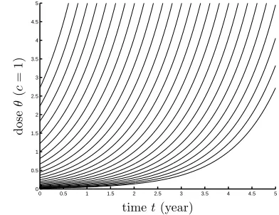
Remark 2.11. The expressions ofS and I in Corollary 2.10 can be viewed as a consequence of a change of variables using the characteristics of the transport part of the PDEs. These characteristics are given by

_˙

a= 1,

˙

θ=c θ,

which suggests the change of variables (t, a, θ)7→(t, b, d) where

a=t−b,

θ=ec(t−d).

This change of variable has the following biological meaning : the variableb denotes the birth date and the variableddenotes the death date.

(12)

0 0.5 1 1.5 2 2.5 3 3.5 4 4.5 5 0

0.5 1 1.5 2 2.5 3 3.5 4 4.5 5

PSfrag replacements

timet(year)

age

a

doseθ (c= 1) 00 0.5 1 1.5 2 2.5 3 3.5 4 4.5 5

0.5 1 1.5 2 2.5 3 3.5 4 4.5 5

PSfrag replacements

timet(year) agea

dose

θ

(

c

=

1)

Figure 1. _{Characteristic curves}

3. Conclusion

The mathematical analysis performed in this paper is a necessary step before tackling parameter estimation on real life data. This type of structured population model is indeed representative of biological phenomenon since it is a simplified version of a multi-genotype model of scrapie transmission that has already been used in [13]. The results presented in this paper are currently beeing extended to the multi-genotype case for further parameter estimation.

Appendix

Proposition 3.1. Letf ∈D(ΦI). The functionGdefined by

G(t, a, θ) :=



 

 

f(a−t, θ e−ct₎_e−(µ+c)t₋_f₍_{a, θ}₎

t t6= 0,

ΦIf(a, θ) t= 0,

is continuous on EI ={(t, a, θ)∈[0,+∞[×[0, A]×[0,1], a≥t}.

Proof. Clearly ΦI(D(ΦI))⊂C((0, A]×[0,1]), thenGis continuous outside the linet= 0 and on the linet= 0. Let us prove that Gis continuous at the junction.

We consider a sequence{(tn, an, θn)}n≥0of EI such that

lim

n→+∞(tn, an, θn) = (0, a, θ)∈ EI,

and we denote by ϕ the smooth map ϕ : (t, a, θ) 7→ (a−t, θ e−ct_{). The function} _f _◦_ϕ _{is C}1_{, and Taylor}

approximation gives

(f_◦ϕ)(tn, an, θn) = (f◦ϕ)(0, an, θn) +D(0,an,θn)(f◦ϕ)(tn,0,0) +o(|tn|),

that we can write, using expressions ofDϕ(0,an,θn)f andD(0,an,θn)ϕ,

(13)

Sincef _∈D(ΦI), we have

lim n→+∞

f(an−tn, θne−ctn)−f(an, θn)

tn

=−∂af(a, θ)−c θ ∂θf(a, θ),

and we can conclude for the continuity by noticing that

G(tn, an, θn) =e−(µ+c)tn

f(an−tn, θne−ctn)−f(an, θn)

tn

+f(an, θn)

e−(µ+c)tn

−1

tn

,

which converges on

−∂af(a, θ)−c θ ∂θf(a, θ)−(µ+c)f(a, θ) =G(0, a, θ).

Proposition 3.2. For allu˜1, u˜2∈ F, we have kFSu˜1(t)−FSu˜2(t)kS ≤

√

A β t(kS0k2S+knk2L2₍₀ ,T))

1

2 sup

t∈[0,δ]k

˜

u1(t)−u˜2(t)kX ∀t∈[0, δ]. (12)

Proof. Using the inequality|e−x₋_e−y_{| ≤ |}_x₋_y_|_for_{x, y}_≥_{0 and expression of}_K₍_I_{) we obtain}

kFSu˜1(t)−FSu˜2(t)k2S ≤

Z min(t,A)

0

β n(t−a)

Z t

t−a

K( ˜I1−I˜2)(u)du

2 da + Z A

min(t,A)

β S0(a−t)

Z t

0

K( ˜I1−I˜2)(u)du

2 da.

Using Cauchy-Schwarz we haveK( ˜I1−I˜2)(u)≤ √

AkI˜1−I˜2kI, and fora≤t

Z t

t−a

K( ˜I1−I˜2)(u)du

≤

t√A sup t∈[0,δ]k

˜

I1−I˜2kI,

and fort≥a

Z t 0

K( ˜I1−I˜2)(u)du

≤

t√A sup t∈[0,δ]k

˜

I1−I˜2kI.

Then

kFS(˜u1(t)−FSu˜2(t)k2S ≤t2β2A

Z min(t,A)

0 |

n(t₋a)|2 da+

Z A

min(t,A) |

S0(a−t)|2da

!

sup t∈[0,δ]k

˜

I1−I˜2kI

!2

,

and (16) consequently.

Proposition 3.3. Letu˜_∈C([0, τ], X)satisfyingu˜(t) =Fu˜(t)on[0, τ]. Then u˜can be extended on[0, τ +δτ_]

where

δτ<min

(

T −τ, 1

2m(rτ_{, T}₎,

1

β√A(knk2

L2₍₀_,T₎+kS˜(τ) +B(τ)nk2_S) 1

2 +m(rτ, T)

)

,

with rτ_{:= 2 (}_k_S

0kS+knkL2₍₀

(14)

Proof. We denote ˜u= ( ˜S,I˜) the solution on [0, τ]. We define the mapping

Fτ: C([τ, τ+δτ], X)→C([τ, τ+δτ], X),

by

Fτ˜uτ(t) :=

Fτ

Su˜τ(t)

Fτ Iu˜τ(t)

:= gτ(t)−B(t)n

TI(t−τ) ˜I(τ) +

Rt

τ TI(t−s) ˜PI(s,u˜

τ₍_s₎₎_ds

!

,

where

gτ(t) :a7→



  

  

˜

S(τ, a−(t−τ)) + (B(τ)n)(a−(t−τ))

×e−(µ(t−τ)+βRτtK( ˜Iτ)(s)ds) _if

a≥t−τ , n(t₋a)e−(µa+β

Rt

t₋aK( ˜Iτ)(s)ds)

ifa_≤t₋τ .

Let us prove that Fτ _{preserves the closed subset}_Fτ _{defined by}

Fτ:=nu˜τ= ( ˜Sτ,I˜τ)∈C([τ, τ+δτ], X),_ku˜τ_kX _≤rτ,S˜τ(t) +B(t)n_≥0 and ˜Iτ(t)≥0o,

andFτ _{is a contraction mapping on}_Fτ_. For ˜uτ_{∈ F}τ _{we have, since}_k_T

I(t)k ≤1,

kFτu˜τ(t)kX≤ kg(τ, a₋(t₋τ))kS+ sup t∈[0,T]k

B(t)n_kS+kI˜(τ)kI+

Z t

τ

rτm(rτ, T)ds

≤ kS0kS+knkL2₍₀_,T₎+ sup t∈[0,T]k

B(t)n_kS+kI˜(τ)kI+ (t₋τ)rτ_m₍_rτ_{, T}₎_,

and using the definition ofδτ_,

kF˜u(t)kX≤rτ.

Moreover, we can check easilyFτ

Su˜τ(t) +B(t)n≥0 and then ˜PI(s,u˜τ(s))≥0. Since ˜I0≥0 andTI is a positive semigroup, we can conclude Fτ

Iu˜τ(t) ≥ 0 and Fτ preservesFτ. Now, let us prove that Fτ is a contraction mapping. Doing the same than in the proof of Proposition 3.2 in appendix, we can see that for ˜u1,u˜2∈ Fτ and

for allt_∈[τ, τ+δτ_],

kF_Sτu˜1(t)−FSτu˜2(t)kS

≤√A β(t₋τ) (kS˜(τ) +B(τ)n_k2_S+kn_k2_L2₍₀ ,T))

1

2 sup

t∈[τ,τ+δτ_]k

˜

u1(t)−u˜2(t)kX. (34)

Furthermore for allt_∈[τ, τ+δτ_]

kFIu˜1(t)−FIu˜2(t)kI ≤

Z t

τ k ˜

PI(s,u˜1(s))−P˜I(s,u˜2(s))kI ds

≤m(rτ, T) (t−τ) sup t∈[τ,τ+δτ_]k

˜

u1(t)−˜u2(t)kX. (35)

With (34) and (35) we have for allt∈[τ, τ+δτ]

sup t∈[τ,τ+δτ_]k

Fu˜1(t)−Fu˜2(t)kX≤

m(rτ, T) +√A β(kS0k2S+knk 2 L2₍₀_,T₎)

1 2

δ

× sup

t∈[τ,τ+δτ_]k

˜

u1(t)−u˜2(t)kX,

(15)

References

[1] O. Arino. A survey of structured cell population dynamics.Acta Biotheoretica, 43:3–25, 1998.

[2] O. Arino, A. Bertuzzi, A. Gandolfi, E. S´anchez, and C. Sinisgalli. A model with ‘growth retardation’ for the kinetic heterogeneity of tumour cell populations.Math. Biosciences, 206:185–199, 2007.

[3] J. Dyson, R. Villella-Bressa, and G.F. Webb. Asynchronous exponential growth in an age structured population of proliferating and quiescent cells.Math. Biosciences, 177–178:73–83, 2002.

[4] H. O. Fattorini. Boundary control systems.SIAM J. Control & Opt., 6(3):349–385, 1968.

[5] D. Givon, R. Kupferman, and A. Stuart. Extracting macroscopic dynamics : model problems and algorithms.Institute of Physics Publishing, Nonlinearity, 17:R55–R127, 2004.

[6] W. O. Kermack and A. G. McKendrick. A contribution to the mathematical theory of epidemics.Proc. Roy. Soc., A, 115:700– 721, 1927.

[7] W. O. Kermack and A. G. McKendrick. Contributions to the mathematical theory of epidemics. II.– The problem of endemicity. Proc. Roy. Soc., A, 138:55–83, 1932.

[8] W. O. Kermack and A. G. McKendrick. Contributions to the mathematical theory of epidemics. III.–Further studies of the problem of endemicity.Proc. Roy. Soc., A, 141:94–122, 1933.

[9] J. D. Murray.Mathematical Biology. Springer, 2002.

[10] A. Pazy.Semigroups of Linear Operators and Applications to Partial Differential Equations. Applied Mathematical Sciences 44. Springer, 1983.

[11] I. Segal. Non-linear semi-groups.Annals of Mathematics, 78:339–364, 1963.

[12] S. M. Stringer, N. Hunter, and M. E. J. Woolhouse. A mathematical model of the dynamics of scrapie in a sheep flock.Math. Biosciences, 153(1–2):79–98, 1998.