Gabriel Caloz & Monique Dauge, Editors
RESOLUTION OF EMC PROBLEMS USING 3D TIME DOMAIN METHODS
Alain Reineix,Christophe Guiffaut, Francis Denanot
1Abstract. Nowadays the number of boarded electronic devices is increasing and simultaneous, the number of electromagnetic perturbations also increases. Then, it becomes necessary to protect these equipments. This domain particularly concerns the ElectroMagnetic Compatibility where the problem is to find solutions to realize a cohabitation between all systems without interferences. As experiments are often expensive and limited, the theoretical approach is a good alternative. The choice of time domain methods is imposed by the nature of the perturbations which are generally transient pulses. So, in this paper, we will present some modelling problems in this area and propose some solutions.
R´esum´e. De nos jours, on assiste `a une augmentation du nombre de syst`emes ´electroniques em-barqu´es. Parall`element, le nombre de perturbateurs potentiels ne cesse de croˆıtre. Ce type de probl`eme concerne le domaine de la compatibilit´e ´electromagn´etique ´etudie plus particuli`erement les probl`emes de cohabitation des syst`emes avec tous les parasites ´electromagn´etiques. Les exp´erimentations ´etant souvent coˆuteuses et limit´ees, une solution alternative est la simulation num´erique. Le choix des ap-proches temporelles est naturel de par l’aspect transitoire d’un grand nombre de perturbations. Dans cet article, nous allons pr´esenter quelques probl`emes de mod´elisation dans ce domaine et ainsi que proposer des solutions potentielles.
Introduction
Nowadays, in the design of electronic equipment, it is necessary to take into account the EMC (Electro-Magnetic Compatibility) problems for different reasons, the main one being the overall decrease of activation levels and the higher integration of components that lead to the increased sensitivity of electronic equipments to electromagnetic parasitics. Added to that, the number of intentionnal and non intentionnal perturbations is strongly increasing - mostly because of the wireless communications expension, and the electronic equipments are now numerous for boarded applications such as in automotives and aeronautic domains. And obviously, in such sensitive areas, dysfunctions are not permitted because dramatic consequences can occur.
In the conception of complex systems, from an economic point of view , it becomes necessary to get infor-mations on the susceptibility levels before the conception of a prototype. So, one of the best solution is the numerical simulation. But, when simulating physical phenomena, it is very important to include all impor-tant behaviours of devices. Due to the increasing capacity of computers and the improvement of numerical methods during the last twenty years, it is now possible to model complex structures included in a cube of ten wavelengths side. But, if we take a closer look to realistic systems, it can be observed that they are generally constituted of some subsystems of different dimensions. As a consequence, as it will be shown in this paper, a multiscale aspect has to be considered. As it will be pointed out, dealing with this problem, involves going from the macroscopic to the microscopic domains, to get the components level on the PCBs (Printed Circuit
1 Xlim,D´epartement OSA, Facult´e des sciences, 123 avenue Albert Thomas 87 060 Limoges Cedex France
c
EDP Sciences, SMAI 2007
Boards).In a second part, we will see how to include such elements in time domain codes. Finally, it will be discussed of an important perturbation which is the lightning.
The electromagnetic problems can be solved in time domain by three kind of 3D methods, all these approaches start from Maxwell’s equations. Rewriting these equations in different forms leads to different approaches to solve them :
-using the differential form of Maxwell’s equation, a centered differentiation allows to use the FDTD method, which calculates E and H fields using an iterative approach limited by a stability criterion,
-writing Maxwell’s equations in a conservative form allows to solve problems using the Finite Volume approach which comes from the fluid dynamics
-a variational form of these equations is generally solved using the Finite element method.
In the time domain and for electromagnetic field problems, the FDTD method has been extensively used for a long time, so, numerous models have been developed. In this paper, we will focus on this approach to solve the different problems quoted above.
1.
Multiscale resolution using a subgridding approach
One of the most illustrative problem of today’s multiscale aspect of EMC is the penetration of parasitic waves inside automotives. When an EM wave arrives on a vehicle, a coupling with the metallic parts is responsible of a parasitic current flowing on the structure. This current is then guided by the cables and arrives on the boarded computers situated inside metallic or dielectric shielding. The perturbation is then coupling to the PCB traces and this can induce dysfunctions in the components connected to the traces. This typical example shows the different scales of the problem, starting from the vehicle down to the components located on the PCB. In this paper, it will be shortly discussed how to solve such problems with a two levels example using a sub gridding method.
If we consider a three dimensional FDTD volume with a structure made of large parts and little details, two spatial steps will be considered : a large one and a refined one. To allow the EM field to propagate between the two regions, a great care has to be taken at the considered interface. Different ways for connected the two grids have been investigated by computing the E field (resp the H field) on the interface using some interpolations. The time step must also be refined in the second region by the same factor. Some of the different solutions encountered in the literatures are for example:
- a linear interpolation to find the E (resp H) tangential components of the fields along the interface. Some papers dealing with this problem have been published for 2D and 3D problems [1,2].
- a spline cubic interpolation for the derivation of the fields at the interface [3]. In order to increase the stability, some other authors have included the resolution of the wave equation at the boundary level. Different ways have been tested to improve the method, leading to the VSSM method [4] and the MRA approach [5].
2.
Linear and non linear components representation in FDTD codes
The transient 3D methods are often used to compute wave diffraction by structures whose dimensions are about some wavelengths. Generally speaking, it is very powerful for dealing with distributed structures. But when considering the computation of parasitic currents flowing on PCB (Printed Circuits Boards), it is important to have a three dimensional discretization of the traces, but the current levels heavily depend on the lumped circuits at the traces’ termination. As due to the current behaviour of linear and non linear circuits, a strong hybridization between the circuit part (lumped part) and the distributed one is needed. So, we deal with some approaches to include the dipoles located at the traces extremities. Usually, for very simple circuits, the Maxwell equations are modified by adding a current density following the I=f(V) law of the element [8,9].It is the case for resistors, capacitors and inductors. When more complicated linear and specially when non linear circuits are dealed with, the approach become instable in some cases. To stabilize the solution, the authors use in most cases a Newton Raphson procedure. A better solution for having stable results is to solve the state variables of the circuit, and to integrate the time domain solution using a Runge Kutta procedure that can be coupled to Fehlberg coefficients. The problem is in the automation of the procedure because, with such an approach, we need to redefine the equations for every particular circuits. So, to overcome these drawbacks in this paper, an original approach will be dealed with. This approach, recently proposed in the litterature for linear circuit, has been extended to non linear components. The different steps to solve a problem with a linear lumped element will be now described. Considering a simple one port linear circuit, it can be assimilated to a dipole and its behavior can be described in the Laplace domain as a Pade rational fraction.
Z(s) =
PM m=0bms
m PM
m=0ams
m W here s is the Laplace domain variable.
The problem with this model is to determine the coefficients of the rational fraction, as they must have some physical properties to get a passive(positive coefficient) and stable impedance ( position of the poles in the right side of the complex plane). So, it is important to have a good fitting method, one of the most appropriate is the Vector Fitting approach presented by Gustavsen [10]. The second point is to transform the continuous problem in the discrete domain, Pereda [11] has proposed to use a well known signal processing method : the z transform. A bilinear transform is used to go from the Laplace domain to the z domain. This transformation automatically gives the bandwidth of interest through the time step△t; the formula connecting the two domains is : s = 2
△t
1−z−1
1+z−1. After some algebraic manipulation, it is easy to derive another rational
fraction which corresponds to a ratio between a current density and an electric field : J(s) =σ(s)E(s)
σ(s) = △x △y△z
PM m=0ams
m PM
m=0bms
m σ(z) =
1 +PMk=1ckz−
k PM
k=0dkz−
k
After the multiplication of the two terms by the denominator and an inverse Z transform, we derive an equation connecting the delayed field components with the delayed current densities. Finally, it has been shown by the authors, that a decomposition in recursive equations can be performed easily. As a consequence, no convolution product has to be solved in the new system. This kind of approach has recently been extended to non linear elements by considering the linear part as a quadrupole and the non linear part by the equivalent circuit. The example shown in the previous quoted paper of a mosfet has given excellent results. Some interesting approaches to perform the resolution avoiding the convolution producted have been proposed by Shao and al [12] and by Wu and al [13].
3.
Lightning modeling
field can disturb different systems in a large area around the impact point. As it will be pointed out, two critical points are encountered for the modelling in the time domain, and they will be developed in the following; it concerns : the time radiation field formulation of the lightning channel and the radiated wave in FDTD codes.
3.1.
Channel modeling for a cloud / ground lightning
In the particular case of a lightning between a cloud and the ground, the modelling of the EM field must start from physical phenomena : as it is well known, a lightning leader is generated and is propagated step by step from the cloud towards the earth. The role of the lightning leader is to create a kind of plasma conductor. When the lightning leader is about 50 meters above the ground, a return stroke is generated because the field is greater than the disruptive air field limit of air. At this moment, the lightning phenomenon is generated, so a strong transient current starting from the ground is flowing in the vertical antenna constituted by the plasma tube. As a consequence, one way for a correct modelling is to consider the channel as a vertical monopole fed by a current generator at its base. As some analytical models are available, such as the Heidler formula, the channel can be represented as a succession of elementary dipoles, the number of dipoles (height of the channel) depending on the observation distance and the observation duration. In order to access to the radiated field in the time domain at observation points, the current contribution of each elementary dipole is integrated over the channel length. When the ground is considered as perfect conductor, this assumption greatly simplifies the radiation formulation of vertical dipole, since only direct wave and perfect image wave from each dipole is treated by well-known relations [15]. Realistic ground with a finite conductivity complicates the evaluation because Sommerfeld integration is the starting point. However, Cooray and Rubinstein [16,17] show that the vertical electric field and the azimutal magnetic field over the poorly conducting ground are not dependent of the conductivity value. So, for these components, the assumption of the perfect conductor ground can be applied in this particular case. Only horizontal electric field over the ground needs a suited relation taking account the exact ground conductivity [15,16]. For the underground electromagnetic fields Cooray [17] proposed some relations for all components of the existing field in the time domain whereas, more recently, Yang & Zhou [18] proposed simple relations (but in the frequency domain) based on a quasi-image formula.
3.2.
Generation of the incident field
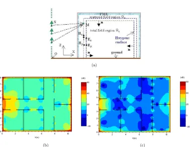
As the radiated field from the lightning channel can be calculated in each point of the space, the problem is now to treat the coupling with a structure discretized in a FDTD volume. The height of the channel and its distance to the structure forbid the inclusion of the channel in the modelling. This can be achieved using a closed Huygens surface surrounding the structure (figure 1a). Up to now, FDTD method uses the Huygens principle for rigorous plane wave illumination inside a closed surface [19]. Retaining a similar algorithm, plane wave radiation formulation is replaced by the elementary dipole radiation relation. Nevertheless, more complex algorithm has to be developed because the field magnitude must be computed for each position. Furthermore, the number of dipoles can be significant, several tens or hundreds, depending on the channel height and the elementary dipole length [20]. To avoid overgrown computationnal times, two main optimizations are proposed to provide low computational effort compared to the field calculation treated by the FDTD method. First, the number of dipoles is minimized using the Shannon criterion : from the maximal frequency of the spectral response, the minimal wavelength that gives an overestimation of the dipole length is deduced : dl lower than 0.5 minimal wavelength.
(a)
(b) (c)
Figure 1. (a) Coupling between a Huygens surface inside the FDTD volume and a channel outside the volume. (b) Magnetic field magnitude in dBA/m (H*120*pi), inside a building inclosure of size 10m*7.5 m* 3 m, T=0.5 us equivalent channel contribution of 40 m, maximum magnitude of the field around the enclosure, aperture to the left side in reinforced concrete face to the corridor. (c) same as (b) with T=1.5 us equivalent channel contribution of 150 m
cells in each axis direction instead of every cells of the Huygens surface. All fields obtained by interpolation have negligible computation time. Consequently and according to the algorithm form, radiated field computational gain will be superior to N and inferior to N*N. With an optimised algorithm, the gain gets close to the upper limit N*N. Figure 1b and 1c illustrate the implementation of the coupling between return stroke and FDTD method for the realistic illumination of a building enclosure with reinforced concrete wall and inner partition. They represent two temporal photographs of the magnetic field, and they show that the main field contribution is provided by the bottom of the channels In this case, a gain of 50 on the sources computation time has been observed.
4.
Conclusion
each case, some particular developments are necessary; for doing this, we need to improve numerical methods, such as the FDTD, which is one of the most versatile one.
5.
References
[1] I.S. Kim and W.J.R. Hoefer, “ A local refinement algorithm for the time-domain finite-difference method using Maxwell’s curl equations” IEEE Trans. Microwave Theory and Tech., vol.38, pp. 812-815, June 1990.
[2] D. T. Shimizu, M. Okoniewski and M. A. Stuchly, “ An efficient subgridding algorithm for FDTD”, in Conf. Proc. 11th Ann. Rev. Progress. Appl. Computat. Electromagn., Monterey, CA, Mar.1995, pp. 762-766. [3] M. Okoniewski, E. Okoniewska and M. A. Stuchly, “ Three-dimensional subgridding algorithm for fdtd”, IEEE Trans. Antennas Propagat. vol 45, pp 422-429, 1997.
[4] S. S. Zivanovic, K. S. Yee, and K. K. Mei, “ A subgridding method for the time-domain finite-difference method to solve Maxwell’s equations,” IEEE Trans. Microwave Theory Tech., vol 39, pp 471-479, Mar. 1991.
[5] D. T. Prescott and N. V. Shuley, “ A method for incorporating different sized cells into the finite-difference time-domain analysis technique,” IEEE Microwave Guided Wave Lett., vol.2, pp. 434-436, Nov.1992.
[6] guiffaut
[7] T. Fouquet, “ Raffinement de maillage spatio-temporel pour les equations de Maxwell, “‘ These de doctorat de Paris IX Dauphine, Juin 2000.
[8] W. Sui, D. A. Christensen, C. H. Durney, “ Extending the Two-Dimensional FDTD Method to Hybrid electromagnetic Systems with active and passive lumped elements” IEEE Tran. on Microwave Theory and Techn., vol. 40, n.4, April 1992, pp 724-422.
[9] C.S. Aitchison et al., “Lumped-circuit elements at microwave frequencies,” IEEE Trans. Microwave Theorytech., vol. 19, no. 12, pp. 928-937,1971.
[10] B. Gustavsen, A. Semlyen, “ Rational approximation of frequency domain responses by vector fitting” IEEE Trans. On Power Delivery, vol.14, n.3, July 1999.
[11] J. A. Perada, F. Alimenti, P. Mezzanotte, L. Roselli, and R. Sorrentino, “ A new algorithm for the incorporation of arbitrary lumped networks into FDTD simulators,” IEEE Tran. Microwave Theory and Techn., vol. 47, n. 6, June 1999.
[12]Z. Shao and M. Fujise, “ An improved FDTD formulation for general linear lumped microwave circuits based on matrix theory” IEEE Trans. Microwave Theory and Tech., Vol. 53, n 7, June 2005.
[13] T. L. Wu, S. T. Chen, and Y. S. Huang, “ A novel approach for the incorporation of arbitrary linear lumped network into FDTD method,” IEEE Microwave and Wireless Component letters, vol 14, n 2, February 2004
[14]M. Rubinstein, ”Transient electric and magnetic fields associated with establishing a finite electrostatic dipole, revised,” IEEE Trans. on Electromagnetic Compatibility, Vol. 33, n4, pp. 312-320, November 1991.
[15]M. Rubinstein, ”An approximate formula for the calculation of the horizontal electric field from lightning at close, intermediate and long range,” IEEE Trans. on Electromagnetic Compatibility, Vol. 38, n3, pp. 531-535, August 1996.
[16]V. Cooray, ”Some considerations on the ”Cooray-Rubinstein” formulation used in deriving the horizontal electric field of lightning return strokes over finitely conducting ground,” IEEE Trans. on Electromagnetic Compatibility, Vol. 44, n4, pp. 560-566, Nov. 2002.
[17]. Cooray, ”Underground electromagnetic fields generated by the return strokes of lightning flashes,” IEEE Trans. on Electromagnetic Compatibility, Vol. 43, n1, pp. 75-84, Feb. 2001.
[18]C. Yang and B. Zhou, ”Calculation methods of electromagnetic fields very close to lightning,” IEEE Trans. on Electromagnetic Compatibility, Vol. 46, n1, pp. 133-141, Feb. 2004.
[19]A. Taflove, S. C. Hagness, ”Computational electrodynamics, the finite difference time domain,” Seco]Edition, Artech House, chapt.5, 2000.