Maximum Power Point Tracking Using State-dependent Riccati equation based Model Reference Adaptive Control

Vol. 3, No. 2, pp. 115-124, April (2020)

Maximum Power Point Tracking Using a

State-dependent Riccati Equation-based Model

Reference Adaptive Control

Mostafa Rahideh

1

, Abbas Ketabi

2,†

, and Abolfazl Halvaei Niasar

3

1,2,3 _{Faculty of Electrical and Computer Engineering University of Kashan, Kashan, Iran}

The present paper proposes an adaptive control method for maximum power point tracking (MPPT) in photovoltaic (PV) systems. To improve the performance of the MPPT, the study develops a two-level adaptive control structure that can facilitate system control and efficiently handle uncertainties and perturbations in the PV systems and in the environment. The first control level is a ripple correlation control (RCC), and the second is a model reference adaptive control (MRAC). The paper emphasizes mainly on designing an MRAC algorithm that improves the underdamped dynamic response of the PV system. The original state-space equation of the PV system is time-varying and nonlinear, and its step response contains oscillatory transients that damp slowly. Using the extended state-dependent Riccati equation (ESDRE) approach, an optimal law of the controller is derived for the MRAC system to remove the underdamped modes in the PV systems. An algorithm of scanning the P-V curve of the PV array is proposed to seek the global maximum power point (GMPP) in the partial shading conditions (PSCs). It is shown that the proposed control algorithm enables the system to converge to the maximum power point in partial shading conditions in milliseconds.

Article Info

Keywords:

Partial shading conditions, PV systems,

Model Reference Control, Ripple correlation control, State-dependent Riccati equation

Article History:

Received 2019-01-20

Accepted2019-09-24

I.

I

NTRODUCTION

Photovoltaic systems are a vital element in achieving national goals of energy independence and decreasing potentially harmful environmental effects caused by an increase in the consumption of fossil fuels. Because of changes in solar irradiance and ambient temperature, photovoltaic systems are constantly unable to provide their optimal power unless an MPPT algorithm is employed. Photovoltaic systems need an MPPT algorithm to adapt to environmental changes and deliver optimal power. In general, MPPT algorithms use power electronic converter systems where the converter duty cycle is controlled to transmit the maximum available power [1], [2].

Many MPPT algorithms have been proposed in the literature. The most common one is perturb and observe (P&O) [3]-[5]. This strategy needs an external circuit that frequently perturbs the voltage of the array and measures the resulting variations in the output power. In spite of the simplicity and lower costs of the P&O algorithm, it is ineffective in the steady-state because it forces the system to swing around the maximum power point. Besides, this algorithm is inefficient under rapidly changing environmental conditions since it cannot distinguish the difference between the variations in power due to environmental effects and the changes in power due to the inherent perturbation of the algorithm [6]. The incremental conductance (INC) technique is based on the fact that the derivative of solar array power is ideally zero at the maximum power point, positive to the left of this point, and negative to the right of this point. It is shown that the INC technique works well in rapidly changing environmental conditions but at the expense of increasing the response time due to the need for

A

B

S

T

R

A

C

T

†_{Corresponding Author: [email protected]}

complex hardware and software [7].

The fractional open-circuit voltage (FOCV) method utilizes an estimated relationship between open-circuit voltage (VOC) and array voltage (Vm) where the maximum power is attained to track the maximum power point [8].

Similar to P&O, the FOCV algorithm is low-cost and can be implemented in a relatively simple manner. However, the FOCV technique is not an exact MPPT because the relationship between VOC and Vm is just an approximation. Neural network and fuzzy logic-based algorithms have shown rapid convergence and high performance under different environmental conditions, but the implementation of these algorithms my turn out to be very complicated [9], [10].

Many papers have proposed optimization algorithms such as artificial bee colony [11], chicken swarm [12], PSO [13,14] and win-driven optimization [15] as an MPPT controller. The accurate tracking of maximum power point (MPP) and slow convergence to the MPP can be enumerated as the main advantage and disadvantage of these methods, respectively.

Many papers have proposed neural network (NN) and fuzzy logic (FL) as an MPPT [16-18]. In these papers, NNs and FLs are used as an adaptive tracker to generate the duty cycle of a DC-DC converter. In spite of the satisfactory performance of these methods, NNs need offline training which is difficult in practice and FLs depend on the knowledge of the designer.

The main problem of MPPT algorithms is transient oscillations in the output voltage of the system after rapidly changing the duty cycle [7]. Therefore, an ideal MPPT algorithm is straightforward and low-cost and shows a rapid convergence to the maximum power point (MPP) with minimum oscillations in the array output voltage.

This paper proposes a two-level control MPPT algorithm which comprises a ripple correlation control (RCC) [19]-[22] at the first level and a model reference adaptive control (MRAC) [23], [24] at the second level. At the first control level, the RCC unit accepts the array voltage and power operate as inputs. The RCC unit then computes the system duty cycle to deliver the maximum power to the load in the steady-state. At the second control level, the MRAC uses the new duty cycle calculated by the RCC unit to improve the dynamics of the photovoltaic power conversion system or the power plant, and eliminate any transient oscillations in the output voltage of array.

As was already mentioned, transient oscillations in the output voltage of the system are created after updating the duty cycle following rapidly changing environmental conditions. To eliminate such oscillations, a critically damped system is selected as the reference model. The proper tuning of the controller parameters causes the output of the system to match the reference model output, where the error converges to zero and the maximum power is attained. Both theoretical and simulation results show convergence to the optimal power point by eliminating underdamped responses, which are frequently observed in photovoltaic power converter systems.

This paper mainly focuses on the MRAC level of the proposed control architecture. In the proposed MRAC, an extended state-dependent Riccati equation (ESDRE) forces the system to track the output of the model reference control.

II.

D

ESCRIPTION OF STATE

-

DEPENDENT

R

ICCATI EQUATION

(SDRE)

Suppose that there is a time invariant nonlinear system and observable as follows:

 

 

x f x G x u (1)

where n

x R are state variables and uRm is the input of the system. Without the loss of generality, it is assumed that f(0) = 0. The nonlinear system given in Eq. (1) can be written in the following pseudo-linear form:

 

 

x A x x B x u (2)

where f(x) = A(x)x and G(x) = B(x). In Eq. (2), A(x) and B(x) are the state-dependent coefficient matrices that represent the nonlinear systems in the form of Eq. (1) in a pseudo-linear form. These matrices are not unique. This is one of the advantages of this technique, which increases the degree of freedom in design. However, it is best to choose the case where matrices A(x) and

B(x) are controllable. The controllability matrix is as follows:

 

 

   

 

 

1

... c x

n

B x A x B x

A x B x

 





 

(3)

A nonlinear system is controllable if the matrix Φ(x) is of full rank for all points.

The purpose of the SDRE is that all state variables reach zero by minimizing the following integral quadratic cost function:

 

 





0

1 2

T T

J x Q x u R x u dt









(4)

where Q x

 

 n n and R x

 

 n m are the state-dependent weight matrices. Both Q and R are assumed to be symmetric and R is positive. These matrices satisfy the following inequality for all x’s:

 

0,

 

0

Q x  R x  (5)

The selection of R and Q has an important role in the performance of the control system. To solve optimal control problems, the Hamilton matrix is used:







 

 



 

 





1 , ,

2

T T

T

H x u x Q x x u R x u

A x x B x u





 

 

(6)

 

 

 

 

 

 

 

0

T T

T

H

x A x x B x u

dA x x dB x u

H

Q x x

x dx dx

H

R x u B x

u



  





   

 _



 _{    }

        

 _

   

    

 _

   

 

(7)

The last equation given in Eq. (7) can be written as:

   

1 T

u R x B x  (8)

By applying the LQR theory, the adjunct matrix is represented by:

 

P x x

  (9)

Finally, the control effort is obtained as:

     

1 T

u R x B x P x x (10)

where P(x) is a positive-definite symmetric matrix derived from the solution of the following Riccati algebraic equation.

   

   

   

1

     

0 T

A x P x P x A x

P x B x R x B x P x Q 

  

(11)

To solve the above equation, A(x) and B(x) should be controllable. Because the matrices given in Eq. (11) depend on the state variables, Eq. (11) should be resolved in each time step to calculate the control effort.

Theorem 1. Consider the nonlinear system given in Eq. (1) with u R1

     

x BT x P x x , P(x) is a positive-definite symmetric solution of the state-dependent Riccati equation of Eq. (11). If the pairs {A(x), B(x)} and {A(x), Q1/2_{} are controllable} and observable, the equilibrium point in the origin of the closed-loop system will be local asymptotically stable [25].

III.

D

ESCRIPTION OF THE

PV

SYSTEM

Fig. 1 shows current-voltage (I-V) and power-voltage (P-V) curves of a photovoltaic array for different levels of solar irradiation. The knee of the I-V curve is where the maximum power point of the photovoltaic array is generated (Vm, Im); when

either Vm or Im is achieved, the maximum power Pm is available.

A photovoltaic system can control the current or voltage of solar panels by means of a dc-dc converter to provide maximum permissible power [26], [27]. Fig. 2 displays a general structure to transfer a PV array power to the load. Depending on the application, other power converters are usable instead of the boost converter.

As shown in Fig. 2, the MPPT controller uses the current and voltage of the PV panels to provide the duty cycle d for the switch S. The relationship between the duty cycle and the array voltage is as follows [28]:





2

1

PV PV o

V I R d (12)

where VPV, IPV, and RO are the voltage and current of the PV array

and the equivalent resistance of the load, respectively. As a result,

the purpose is to design an MPPT controller that constantly computes the optimal value of d so that VPV tracks the path of Vm

and thus provides the maximum accessible power.

If there is not a shadow condition, an M-series N-parallel module array generates an output voltage M × Vmpp (where Vmpp

is PV voltage at the maximum power point), an output current N

× Impp (where Impp is PV current at the maximum power point)

and an output power M × N × Pmpp (where Pmpp is PV power at

the maximum power point) at the maximum power point (MPP). According to Fig. 3, if there are variously shaded PV modules in a PV array, the output power is no longer equal to the unshaded case. The variously shaded case causes a multiple peak value problem and disables the maximum power point tracker from finding the MPP.

Fig. 1. The (I-V) and (P-V) curves of photovoltaic systems under various levels of solar irradiation.

Fig. 2. The MPPT controller of a photovoltaic boost converter system.

Fig. 3. A PV array consisting of unshaded and shaded modules.

0 50 100 150 200 250 300 350

0 100 200 300

400 1 kW/m2

C

u

rr

e

n

t

(A

)

Voltage (V)

Array type: SunPower SPR-305-WHT; 5 series modules; 66 parallel strings

0.75 kW/m2

0.5 kW/m2

0.25 kW/m2

0 50 100 150 200 250 300 350

0 5 10

x 104

1 kW/m2

P

o

w

e

r

(W

)

Voltage (V)

0.75 kW/m2

0.5 kW/m2

0.25 kW/m2

IL

LO

IPV

Temperature Irradiance

To utility grid

C

O

S I Rs

+ V

-+

VPV

-Inverter PV

Array

The proposed method

VPV

IPV

A. Exact State-Space Model of Boost Converter

To obtain state equations, the states x1 and x2 are assigned to the current of the inductor LO and the voltage of the capacitor CO,

respectively [29]. According to Fig. 2, we can then write [29]:

1 1

2 2

O PV s

O

O L x V R x V

x C x I

R

  

  (13)

where Rs is the series resistance and according to Fig. 2, V and I

indicate the voltage across the switch and current drawn from the boost converter by the grid, respectively. Now, I and V

should be expressed as functions of the state variables. They can be defined as portions of x2 and xl [29].

 

 

1 2

2 1

V s t x

I s t x



 (14)

where sl(t), s2(t) are the switching functions represented by [29]:

 

 

1 2

2 2

V s t

x I

s t

x





(15)

By placing Eq. (14) in Eq. (13) and rearranging it, the state equation and the output equation of the boost converter can be written as:

 

 

 

x A x x B x

y C x

 

 (16)

where

 

 

 

1

2

, 1

s

O O

O O L

s t R

L L

A x

s t

C C R

  

 

 

  _ 

 

 

 

 

 

1

, 0 0 1

O

L B x

C x

 

 

  

 

 

 _ _

(17)

IV.

P

ROPOSED

MPPT

ALGORITHM

In this paper, a two-level adaptive control algorithm shown in Fig. 4 is considered as the MPPT. In the first control level, the duty cycle d is computed by the RCC. In the second control level, an MRAC controls the dynamical behavior of the boost converter in response to the duty cycle computed from the RCC unit and prevents the oscillations of the array voltage after any rapid change in the solar irradiation. The RCC level is responsible for changes in solar irradiation and the adjustment process of RCC should be fast enough to compensate for changes in the solar system. Therefore, it is necessary for the time constant of the RCC to be smaller than the dynamics of irradiation variations. On the other hand, the MRAC is responsible to keep optimal damping characteristics of the boost converter whose time constant is much smaller than the

environmental changes.

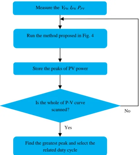
In order to track the maximum power point in the PSC, the algorithm of seeking global maximum power point is drawn in Fig. 5. In this algorithm, the proposed method shown in Fig. 4 is run from the minimum feasible voltage for the PV to the open-circuit voltage of the PV (whole the P-V curve of the PV array). The RCC method scans whole the P-V curve of the PV array and finds multiple peaks. Finally, the greatest peak is the GMPP, and the related duty cycle is selected as the output of the algorithm.

A. RCC method

The key novelty of the RCC is to utilize the switching ripple inherent to perturb the system and therefore track the maximum power point [22]. The RCC method is basically an improved version of P&O [3]-[5] except that the perturbation is inherent to the boost converter.

Fig. 4. The proposed MRAC structure.

Fig. 5. The algorithm to seek the global maximum power point.

+ -

e IPV

VPV

ESDRE

RCC given

Reference model given

in Eq. (20)

Plant given

d*

d

MRAC

up

ym

No Measure the VPV, IPV, PPV

Run the method proposed in Fig. 4

Store the peaks of PV power

Is the whole of P-V curve scanned?

Find the greatest peak and select the related duty cycle

In the RCC method, the product of the time derivative of the array voltage (VPV) and power (PPV) is constantly observed to find out if it is greater than zero to the left side of the MPP, less than zero to the right side of the MPP, and exactly zero at the MPP. 0 when 0 when 0 when PV PV PV M PV PV PV M PV PV PV M dp dv V V dt dt dp dv V V dt dt dp dv V V dt dt       (18)

These observations result in the following control law [19]:

 

PV PV

dd t dP dV

k

dt  dt dt (19)

where k is a negative constant. The control law given in Eq. (19) can be stated as follows: an increase in VPV leads to an increase

in the PPV and since the operating point of the system is to the

left of the MPP, the duty cycle d has to decrease; a decrease in

VPV leads to a decrease in the PPV and since the operating point

of the system is to the right of the MPP, the duty cycle d has to increase. It is clear from Eq. (18) and (19) that the objective is to drive the time-based derivative d to zero to obtain the maximum power. The benefit of the RCC method compared to conventional algorithms such as P&O is that in steady-state, the RCC converges to zero while P&O begins to oscillate around the MPP.

B. Design of an MRAC based on ESDRE

In a boost converter, the response of the converter to the input signal (duty cycle) is highly dynamic. Since the operational point varies with the solar irradiation variations, it is not guaranteed for the voltage of array to show critically damped behavior. Here, the critically damped behavior of the array voltage is maintained by an MRAC based on ESDRE. The basic idea is that the MRAC forces the controlled plant to track the response of the reference model with the desired dynamics in spite of the uncertainties and plant parameters variations. The proposed MRAC structure is depicted in Fig. 3. The input of the total system, d, is the duty cycle calculated by the RCC method. The plant model in Fig. 3 is related to the system given in Eq. (16). The transfer function of the reference model is represented by:

 

 

 

2

m m

m

m m

y s k

G s

d s s a s b

 

  (20)

where km is a positive gain, and am and bm are selected to achieve

a critically damped step response. The proposed extended state-dependent Riccati equation is explained below.

The goal is to design a controller for the system of Eq. (16) such that the system output yp=h(x) asymptotically tracks the

desired value ym. For this goal, the equation q(t) is defined as

follows:

 

m p

q t y y (21)

We assume that the pseudo-linear representation of h(x) is h(x) =C(x) x. Hence, Eq. (21) can be written as:

 

m

 

q t y C x x (22)

By combining Eq. (21) with Eq. (22), we have:

 



  

 

0

, _p n n _m

l

x t A x q x t B x u y

I



 

  _{  }

  (23)

where

 

 

 





 

 

 

 

0 , 0 0 n l l l l m x t x t q t A x A x q

C x B x B x                                (24)

If the weight matrices R n m and Q n l   n l

are positive semi-definite and positive-definite, the following state-dependent Riccati equation will have symmetric positive definite P(x,q) and according to Theorem 1,

    



* 1

,

T p

u d  R x B x P x q x can stabilize the

controlled plant and it is, therefore, possible to say that ypcan

track ym.

   

   

   

1

     

, , , ,

, , T , 0

A x q P x q P x q A x q

P x q B x R x q B x P x q Q



  

(25)

V.

S

IMULATION RESULTS AND DISCUSSION

The MRAC designed in Section V is simulated here for confirmation. The parameters of the boost converter which lead to an underdamped response and controller parameters are provided in the appendix. The array voltage of the plant model (the boost converter) has an underdamped step response, while the step response of the reference model is critically damped. The damping ratio, which is equal to a_m 2 b_m, is a decisive factor as inferred from Eq. (20). It is usually selected to be either slightly less than 1 or exactly 1. In the first case, the step response rises faster along with a slight overshoot.

In addition, the MPPT efficiency at each sampling time Ts is

determined by: 1 1 k k N s k N MPPT s k P T P T      





(26)

where Pk is the PV array power in the presence of the MPPT

controller at the kth sample and PMPPTk is the maximum power

A. The performance of the proposed approach in normal condition

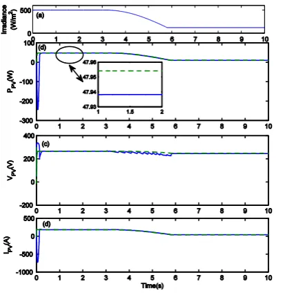
In this test, the goal is to apply several probable linear irradiance trajectory variations to the PV-array. Thus, the trajectory shown in Fig. 6(a) is used. Besides, Figs. 6(b-d) show the MPPT performance of the proposed approach and the conventional P&O algorithm.

As displayed in Fig. 6(a), at t=0.35s, with a steep drop, the irradiance trajectory is set to S=250 W/m2 _{form S=1000 W/m}2_. At t=1.1s, another step in the irradiance increases this level to S=1000 W/m2_{. Two more steep variations drop and rise the} irradiance levels at t=1.65 s and t=2.7 s, to S=500 W/m2 _and S=750 W/m2_{, respectively. From this point onwards, a ramp} variation is also applied to the PV-array. By means of variations, in addition to dynamic behavior analyses, the steady-state behaviors are also assessed.

The voltage and current of PV-array are drawn in Figs. 6(c) and (d), respectively. As is seen in these figures, the oscillatory behavior of the conventional P&O algorithm in tracking the IMPPT is obviously visible. Instead, the proposed approach tracks the reference irradiance level with minimum error. So, the drawn current and active power tracks the reference values smoothly at all times.

In the next test, a sinusoidal irradiance trajectory plotted in Fig. 7(a) is applied to the PV-array. For this simulation, the parameters of the PV system are varied (about 5% of variations). The test results are plotted in Figs. 7(b-d). Clearly, the suggested approach forces the PV-array to track the MPP with minimum error. On the other hand, large amounts of error in PPV, VPV, and IPV can be seen in the results of the conventional P&O algorithm. Once again, the superiority of the proposed approach is verified since the current trajectory is tracked with the least amount of oscillations possible by the proposed approach and consequently, very insignificant active power oscillations are observed. In addition, the performance of the proposed method is robust to parameter variations.

1) A comparative study: This subsection presents a comparative study between the proposed approach and the method proposed in [30]. This reference proposes an improved double integral sliding mode MPPT controller (IDISMC) for a stand-alone photovoltaic (PV) system. The results of the comparison are shown in Fig. 8. As is seen in this figure, the proposed approach makes a better control effort for tracking the maximum power point tracking. Table 1 provides numerical analyses for the two controllers. As is evident in this table, the best performance belongs to the proposed approach.

Fig. 6. Irradiation changes test (a): the irradiance variations (b): active power of the PV-array (c): output voltage of the PV-array (d): output

current of the PV-array; solid (our proposed approach), dashed ([conventional P&O algorithm]).

Fig. 7. Sinusoidal irradiance changes test (a): the irradiance variations (b): active power of the PV-array (c): output voltage of the PV-array (d):

Fig. 8. The results of the comparative study; solid (approach proposed in [30]), dashed ([our proposed approach]).

TABLE I

NUMERICAL ANALYSES FOR OUR PROPOSED APPROACH AND THE METHOD PROPOSED IN [22].

Method Rise time

(s)

Settling time (s)

Efficiency (using Eq.

(26)) Proposed

approach

0.012 0.16 98.82%

[30] 0.038 0.20 96.76%

2) The performance of ESDRE: To demonstrate the independent performance of the ESDRE, a study comparative between in the presence of ESDRE block, in the absence of ESDRE block and the theoretical MPP voltage is displayed in Fig. 9 where a square pulse width modulated signal is the representative of a continuous updating of the duty cycle due to the variance in the solar irradiation. As is evident in Fig. 9, both the unadapted array voltage and the adapted array voltage reach the MPP voltage in the steady-state. This shows the precision of the RCC unit and its capability in computing the optimal duty cycle which can provide maximum power in the steady-state. However, the adapted array voltage has a damped response while unadapted array voltage shows an oscillatory response. Then, at 10 ms, a change occurs in the solar irradiation and the response of unadapted voltage is underdamped and oscillatory. At this point, the adaptive voltage also shows the desired dynamic response. This is one of the purposes of this paper, i.e. to remove any potential underdamped dynamic in the response of the plant due to rapid changes in solar irradiation. The explanations of Fig. 9 are completed in Fig. 10, where the error between the adapted array voltage and the theoretical MPP voltage is drawn. Table II provides the results of comparing different cases in terms of dynamic specifications. As is seen in Table 2, array voltage in the presence of the ESDRE has the

lowest settling time and overshoots while unadapted array voltage has the lowest rise time with most oscillations.

Fig. 9. The comparison of the theoretical MPP voltage, adapted array voltage, and unadapted array voltage.

Fig. 10. The error between the theoretical MPP voltage and the adapted array voltage due to a square pulse-width modulated signal.

TABLE II

THE PERFORMANCE OF ESDRE.

Case Rise time

(s)

Settling time (s)

Overshoot (%) Without

ESDRE block

0.015 0.15 79.16

With ESDRE block

0.055 0.06 0.12

TABLE III

NUMERICAL ANALYSES FOR TWO PSCS.

PSC Convergence time (s)

Settling time (s)

Steady state error (W)

Efficiency (using Eq.

(26)) Two peaks 0.27 0.10 0.2 W 98.68%

Three

peaks 0.35 0.11 0.45 W 97.10%

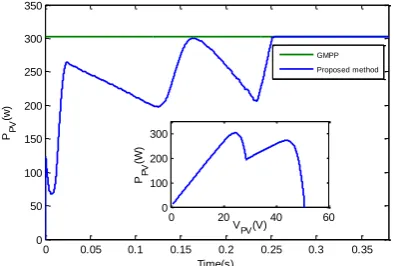
3) The performance of the proposed approach in PSCs: To show the effectiveness of the suggested MPPT controller in partial shading condition, we assume that one shaded PV module receives 200 W/m2 _{and another module receives 400} W/m2_{. According to the P-V characteristic curves drawn in Fig.} 11, there is one global maximum power point and one local maximum power point. It is clear from this figure that the

0 0.05 0.1 0.15 0.2 0.25 0.3 0

50 100 150 200 250 300 350 400 450

Time(s)

A

rr

ay

V

ol

ta

ge

(

V

)

Theoretical MPP Voltage Without

MRAC

With MRAC

0 0.05 0.1 0.15 0.2 0.25 0.3 -400

-300 -200 -100 0 100 200

Time(s)

V

ol

ta

ge

E

rr

or

With MRAC

proposed GMPPT converges to the GMPP with satisfactory accurate.

Fig. 12 shows the performance of the proposed method for a PSC with three peaks. According to the P-V characteristic curve drawn in Fig. 12, the amount of the GMPP is 826.7 W. As can be seen in Fig. 12, the proposed GMPPT has converged to the GMPP with the quickest response and the smallest error.

Table III provides the performance of the proposed method for two partial shading conditions.

Fig. 11. The PV array power at a partially shaded condition with two peaks.

Fig. 12. The PV array power at a partially shaded condition with three peaks.

VI.

C

ONCLUSION

To enhance the efficiency of PV systems, MPPT algorithms are utilized to deliver maximum power from the solar array to the load. Important issues to be considered in designing the MPPT algorithms include the complexity of the system, dynamical performance, and uncertainty. This paper introduces a two-level adaptive control architecture that can reduce complexity in the system control and efficiently handle the uncertainties and perturbations in the PV systems and in the environment. The first level is an RCC, and the second level is an MRAC. This paper focuses mainly on the design of the MRAC algorithm, which improves the underdamped dynamic response of a PV system. Using an optimal law of the controller derived from the extended state-dependent Riccati equation

(ESDRE) approach, the MRAC is capable of removing the oscillatory and underdamped modes in PV systems. The whole of the P-V curve of the PV array is searched by a new algorithm to find the global maximum power point (GMPP) in the partial shading conditions (PSCs) in the presence of multiple peaks. It is shown that the proposed control algorithm enables the system to converge to the maximum power point. The main challenge in implementing the proposed approach is to identify the boost converter parameters which are required in the MRAC design.

A

PPENDIX

ESDRE parameters: Q=diag(0.1,0.1,45), R=1000

Boost converter parameters: Ri=65, Ci=100μF, Lo=5mH, Co=12mF

Model Reference control parameters:

9 3 6

1 10 , 8.17 10 , 2 10

m m m

k   a   b  

R

EFERENCES

[1] S. L. Brunton, C. W. Rowley, S. R.Kulkarni, and C. Clarkson, “Maximum power point tracking for photovoltaic optimization using ripple-based extremum seeking control,” IEEE Trans. Power Electron., vol. 25, no. 10, pp. 2531–2540, Oct. 2010.

[2] R. A.Mastromauro, M. Liserre, T.Kerekes, and A. Dell’Aquila, “A single-phase voltage-controlled grid-connected photovoltaic system with power quality conditioner functionality,” IEEE Trans. Ind. Electron., vol. 56, no. 11, pp. 4436–4444, Nov. 2009.

[3] A. K. Abdelsalam, A. M. Massoud, S. Ahmed, and P. N. Enjeti, “High-performance adaptive perturb and observe MPPT technique for photovoltaic-based microgrids,”

IEEE Trans. Power Electron., vol. 26, no. 4, pp. 1010– 1021, Apr. 2011.

[4] M. A. Elgendy, B. Zahawi, and D. J. Atkinson, “Assessment of perturb and observe MPPT algorithm implementation techniques for PV pumping applications,”

IEEE Trans. Sustainable Energy, vol. 3, no. 1, pp. 21–33, Jan. 2012.

[5] G. Petrone, G. Spagnuolo, and M. Vitelli, “A multivariable perturb-and-observe maximum power point tracking technique applied to a single-stage photovoltaic inverter,” IEEE Trans. Ind. Electron., vol. 58, no. 1, pp. 76–84, Jan. 2011.

[6] S. Jain and V.Agarwal, “A new algorithm for rapid tracking of approximate maximum power point in photovoltaic systems,” IEEE Power Electron. Lett., vol. 2, no. 1, pp. 16–19, Mar. 2004.

[7] N. Femia, G. Petrone, G. Spagnuolo, and M. Vitelli, “Optimization of perturb and observe maximum power point tracking method,” IEEE Trans. Power Electron., vol. 20, no. 4, pp. 963–973, Jul. 2005.

[8] M. A. S. Masoum, H. Dehbonei, and E. F. Fuchs,

0 0.05 0.1 0.15 0.2 0.25 0.3 0.35

0 50 100 150 200 250 300 350

Time(s)

PP

V

(w

)

GMPP Proposed method

0 20 40 60

0 100 200 300

V_PV(V)

PP

V

(W

)

0 0.1 0.2 0.3 0.4 0.5

0 100 200 300 400 500 600 700 800 900

Time(s)

PP

V

(W

)

0 50 100

0 500 1000

V_PV(V)

PP

V

(W

)

“Theoretical and experimental analyses of photovoltaic systems with voltage and current-based maximum power-point tracking,” IEEE Trans. Energy Convers., vol. 17, no. 4, pp. 514–522, Dec. 2002.

[9] Yilmaz, U., Kircay, A., & Borekci, S. (2018). PV system fuzzy logic MPPT method and PI control as a charge controller. Renewable and Sustainable Energy Reviews, 81, 994-1001.

[10] Duman, S., Yorukeren, N., & Altas, I. H. (2018). A novel MPPT algorithm based on optimized artificial neural network by using FPSOGSA for standalone photovoltaic energy systems. Neural Computing and Applications, 29(1), 257-278.

[11] Oshaba, A. S., Ali, E. S., & Abd Elazim, S. M. (2016). PI controller design using artificial bee colony algorithm for MPPT of photovoltaic system supplied DC motor‐ pump load. Complexity, 21(6), 99-111.

[12] Wu, Z., Yu, D., & Kang, X. (2018). Application of improved chicken swarm optimization for MPPT in photovoltaic system. Optimal Control Applications and Methods, 39(2), 1029-1042.

[13] Priyadarshi, N., Azam, F., Sharma, A., Bhoi, A. K., & Kumar, M. (2018). A Particle Swarm Optimization based Fuzzy Logic Control for Photovoltaic System.

International Journal of Engineering & Technology, 7(3.24), 491-496.

[14] Farzaneh, J., Keypour, R., & Karsaz, A. (2019). A novel fast maximum power point tracking for a PV system using hybrid PSO-ANFIS algorithm under partial shading conditions. International Journal of Industrial Electronics, Control and Optimization, 2(1), 47-58.

[15] Abdalla, O., Rezk, H., & Ahmed, E. M. (2019). Wind driven optimization algorithm based global MPPT for PV system under non-uniform solar irradiance. Solar Energy, 180, 429-444.

[16] Assahout, S., Elaissaoui, H., El Ougli, A., Tidhaf, B., & Zrouri, H. (2018). A Neural Network and Fuzzy Logic based MPPT Algorithm for Photovoltaic Pumping System.

International Journal of Power Electronics and Drive Systems, 9(4), 1823.

[17] Duman, S., Yorukeren, N., & Altas, I. H. (2018). A novel MPPT algorithm based on optimized artificial neural network by using FPSOGSA for standalone photovoltaic energy systems. Neural Computing and Applications, 29(1), 257-278.

[18] Haddouche, A., Mohammed, K., & Farah, L. (2018). Maximum Power Point Tracker Using Fuzzy Logic Controller with Reduced Rules. International Journal of Power Electronics and Drive Systems, 9(3), 1381. [19] P. T. Krein, “Ripple correlation control, with some

applications,” in Proc. IEEE Int. Symp. Circuits Syst., 1999, vol. 5, pp. 283–286.

[20] D. L. Logue and P. T. Krein, “Optimization of power electronic systems using ripple correlation control: A dynamic programming approach,” in Proc. IEEE 32nd Annu. Power Electron. Special. Conf., 2001, vol. 2, pp. 459–464.

[21] J. W. Kimball and P. T. Krein, “Discrete-time ripple correlation control for maximum power point tracking,”

IEEE Trans. Power Electron., vol. 23, no. 5, pp. 2353– 2362, Sep. 2008.

[22] T. Esram, J. W. Kimball, P. T. Krein, P. L. Chapman, and P. Midya, “Dynamic maximum power point tracking of photovoltaic arrays using ripple correlation control,”

IEEE Trans. Power Electron., vol. 21, no. 5, pp. 1282– 1291, Sep. 2006.

[23] D. E. Miller, “A new approach to model reference adaptive control,” IEEE Trans. Autom. Control, vol. 48, no. 5, pp. 743–757, May 2003.

[24] S. Sastry and M. Bodson, Adaptive Control: Stability, Convergence and Robustness. New York: Dover Publications, 2011.

[25] Y. Batmani, H. Khaloozadeh, “On the design of human immunodeficiency virus treatment based on a non-linear time-delay model,” IET Systems Biology, 2013,10.1049/iet-syb.(2013).0012.

[26] E. V. Solodovnik, S. Liu, and R. A. Dougal, “Power controller design for maximum power tracking in solar installations,” IEEE Trans. Power Electron., vol. 19, no. 5, pp. 1295–1304, Sep. 2004.

[27] A. D. Rajapakse and D. Muthumuni, “Simulation tools for photovoltaic system grid integration studies,” in Proc. Electr. Power Energ. Conf. (EPEC 2009), Oct., pp. 1–5. [28] A. D. Rajapakse and D. Muthumuni, “Simulation tools for

photovoltaic system grid integration studies,” in Proc. Electr. Power Energ. Conf. (EPEC 2009), Oct., pp. 1–5. [29] Rim, C., Joung, G. B., & Cho, G. H. (1988). A state space

modeling of non-ideal DC-DC converters. In PESC 88 Record 19th Annual IEEE Power Electronics Specialists Conference (1988) (pp. 943-950). IEEE.

Mostafa Rahideh was born in Yasuj, Iran in 1982. He received his B.Sc. in electrical engineering from Shiraz University in 2006 and his M.Sc. in electrical engineering (Power Electronics Engineering) from the Shahrood University of Technology in 2010. Since September 2014, he has been working on his Ph.D. degree at the University of Kashan in electrical engineering. His current major research areas include power electronic and Photovoltaic systems.

Abbas Ketabi received his B.Sc. and M.Sc. degrees in electrical engineering from the Department of Electrical Engineering, the Sharif University of Technology, Tehran, Iran, in 1994 and 1996, respectively. He received his Ph.D. degree in electrical engineering jointly from the Sharif University of Technology and the Institut National Polytechnique de Grenoble (Grenoble Institute of Technology), Grenoble, France in 2001. Since then, he has been at the Faculty of Electrical Engineering, the University of Kashan where he is currently an associate professor. He has published more than 80 technical papers and 5 books. He is the manager and editor of the journal “Energy: Engineering and Management”. Dr. Ketabi received the University of Kashan Award for distinguished teaching and research. His research interests include power system restoration, smart grids, renewable energy, optimization shape of electric machines, and evolutionary computation. (Faculty of Electrical Engineering, the University of Kashan, Based on document published on September 13, 2017)