Joint Allocation of Computational and Communication Resources to Improve Energy Efficiency in Cellular Networks

(1)

Please cite this article as: N. Nouri, A. Entezari, Joint Allocation of Computational and Communication Resources to Improve Energy Efficiency in Cellular Networks, International Journal of Engineering (IJE), IJE TRANSACTIONS B: Applications Vol. 32, No. 11, (November 2019) 1627-1633

International Journal of Engineering

J o u r n a l H o m e p a g e : w w w . i j e . i r

Joint Allocation of Computational and Communication Resources to Improve Energy

Efficiency in Cellular Networks

N. Nouri*, A. Entezari

Cell Lab, Department of Electrical Engineering, Yazd University, Yazd, Iran

P A P E R I N F O

Paper history:

Received 22 October 2018

Received in revised form 30 April 2019 Accepted 03 May 2019

Keywords:

Mobile Cloud Computing Heteregeneous Network Non-convex Function Bandwidth Allocation Convex Approximation

A B S T R A C T

Mobile cloud computing (MCC) is a new technology that has been developed to overcome the restrictions of smart mobile devices (e.g. battery, processing power, storage capacity, etc.) to send a part of the program (with complex computing) to the cloud server (CS). In this paper, we study a multi-cell with multi-input and multi-output (MIMO) system in which the cell-interior users request service for their processing from a common CS. Also, the problem of the optimum offloading is considered as an optimization problem with optimization parameters including communication resources (such as bandwidth, transmit power and backhaul link capacity) and computational resources (such as the capacity of cloud server) in the downlink network. The main goal is to minimize the total energy consumption by mobile users (MUs) for processing with the delay limitation for each use. This issue leads to a non-convex problem and to solve the problem, we use successive convex approximation (SCA) method. We finally show that the joint optimization of these parameters leads to reducing the energy consumption of the network with simulation examples.

doi: 10.5829/ije.2019.32.11b.14

1. INTRODUCTION1

With the increment of technology in mobile devices, popular applications are daily offered to network users which will be more complex and demand heavy computation. Despite enhancing technology in mobile devices and their applications, there are some challenges in their resources such as storage capacity, battery lifetime and computational capacity which restricts the application’s usage. Recently, mobile cloud computing (MCC) has been suggested as an efficient solution to overcome the restriction in mobile devices to benefit from cloud computing (CC) potential in mobile computing (MC) [1-4]. It can be said that MCC is a combination of CC and MC [5]. Employing this method, we can send a part of the program which has complicated computing and difficult calculations, to the cloud server (CS) [6]. The advantage of employing this method is to diminish the amount of energy consumption by mobile users (MUs), which improve the battery lifetime and computing speed [7, 8]. Moreover, using this type of

*Corresponding Author Email: [email protected] (N. Nouri)

processing, MUs do not require to upgrade their mobile devices in terms of hardware and software.

Barbarossa et al. [9] studied a technique for the joint allocation of communication and computation resources in the single-user mode. Besides, the optimal resources allocation in the network is generalized as multi-user form by Barbarossa et al. [9]. Unlike the consideration of centralized structure for CS in literature [9, 10]; Barbarossa et al. [11], Chen [12] consider that the CS has a decentralized structure and they solve the problem of optimal resources allocation via game theory methods.

(2)

non-convex form. Considering a logical and simplistic assumption for solving the problem, we employ a method called successive convex approximation (SCA) in this paper. Extensive simulation studies demonstrate the energy efficiency improvement of our proposed method and the superior performance over several existed schemes.

This paper is organized as follows. In section 2, we provide our system model and formulate the problem of the optimal resources allocation in mathematical form. In section 3, we discuss the proposed algorithm and solve the problem. In section 4, we provide the results using some simulation examples and finally, we conclude the paper in section 5.

2. SYSTEM MODEL

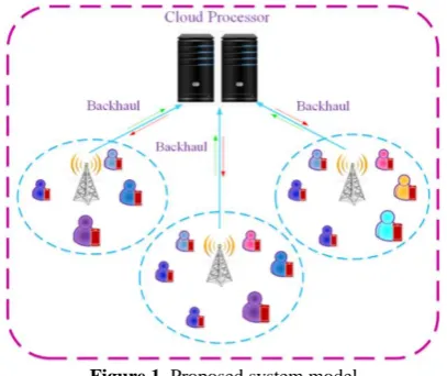
Figure 1. shows the proposed model which is considered a multi-cell network with multi-input multi-output (MIMO) including N_ccell. Moreover, there are M MUs and a base station (BS) in each cell where all BSs are connected to a common server with limited resources. Note that these servers provide computing and storage resources to MUs which is called CSes.

We assume that the backhaul capacity between BS and CS is limited. In addition, MUs in each cell have orthogonal spectral resources, i.e., there is no intra-cell interference between MUs in each cell. However, the effect of the inter-cell interference is considered between MUs of cells with different spectral resources.

Also, we indicate all MUs with the set of



m mn: =1,...,M n, =1,...,Nc



N in which m_n denotes

the MU which uses the spectral resource m in cell n. We also consider the number of the transmitted and received antennas as

mn

T

N and

n

R

N , respectively.

Figure 1. Proposed system model

We denote the application that each MU wants to run as

max

{ , , }

n n n n

I

m = m m m

AP P V B where

n

m

V is required CPU-cycle to run the program. In addition,

n

I m

B and max

n

m



indicate data bits (which includes transmitted code and additional data) and the upper bound of acceptable delay for running the application of each MU, respectively. We define the parameter

n m



as the processing percentage of each MU that transmits to the cloud server.

Therefore, the total delay of each MU will incur for receiving the service is given by:

( )

(

1

)

( )

,

n n n n n

off

m m m m m



• = −





• +

 

• (1)

where

( )

n m



• is the amount of caused delay to process

the program local condition. Furthermore,

( )

n off m



• in (1) denotes the total caused delay for receiving the service from the CS which can be expressed as follows:

,

n n n n n

ul bh exe dl

m m m m m



+



+



+



(2)

where

n ul m



indicates the value of caused delay in

transmitting data from MU m_n to the BS.

( )

n exe m



• is the

delay value that is consumed for computing the program in the CS and

( )

n bh m



• is the caused delay in the backhaul between BS and CS in the downlink direction. Finally,

( )

n

dl m

 • denotes the delay value for sending the transmitted processing results from the CS to the typical MU. Furthermore, energy consumption by each MU to receive the service is given by:

( )

(

( )

) (

1

)

( ),

n n n n n n

ul dl

m m m m m m

e • = e • +e • + − e • (3)

where

( )

n

ul m

e • and

( )

n

dl m

e • denote the energy that is transmitted and received data between typical MU and BS by MU m_n in the uplink and downlink directions, respectively. In addition,

( )

n

m

e • is the energy consumption in the CS condition.

The main purpose of this model is to minimize the total amount of energy consumption by MUs to receive the service with the delay limit constraint. In the sequel, we compute the values of the energy and delay and express the model in mathematical form.

2. 1. Local Processing If we denote the computational capability of each MU in terms of the CPU-cycle per second by

n m

f , the required time for local computing

n

m

(3)

( ) n , ,

n n n

m

m m n

m

f m

f

 =V N (4)

In addition, the required energy for computing can be expressed as:

2

( ) ( ) , ,

n n n n

m m m m n

e f =V f m N (5)

in which



is the effective capacitance of switch which depends on the structure of each MU [15].

2. 2. Uplink Transmission We assume that the transmitted signal from each MU is denoted by

n ul m X

where ul_n

(

, ul_n

)

m CN 0 m

X Q and H

E

n n n

ul ul ul

m =  m m 

Q X X .

Moreover, we express the feasible set of all covariance matrices

n ul m

Q as follows:



Tmn Tmn : 0, ( ) P



n n n n n

N N

ul ul ul ul ul

m m m tr m m



  

Q C Q Q

Q (6)

where P

n ul

m expresses the maximum power of each MU

in the uplink direction. The data transmission rate of the MU m_n in terms of bits/seconds is given by:

2

log det(I H R (Q , )H )

n n n n n n n n

ul ul ul ul ul ul

m m m n m m m m n m

r w − w

 +

= Q (7)

where

, ,

,

( , ) ₀

R Q ΝI + H H

n n n n r r r

r

ul ul ul ul ul

m m m m j n j j n

j r n

w w 

−





N 

Q ₍₈₎

in which Rulm_n(Qul−m_n,wulm_n) is the covariance matrix of the

disturbance (noise plus inter-cell interference) in cell n and mth_{spectral resource. In addition,}

,

H n

m n is the channel matrix between MU m_n and the tagged BS while H _,

r

j n is the channel matrix between the interference MU j_r and the BS in cell n in the uplink case. Ν₀ denotes the power spectral density of the noise and

n ul m

w

denotes the bandwidth that is allocated to the MU m_n in the uplink case. We also have:

( )

(

1

)

_1, . c

n r

N M

ul ul

m j _j

r r n

− ₌

= 

Q Q (9)

The required time for transmitting n

I m

B data bits from MU to the BS can be expressed as:

(

)

2 , ,

log det ( , )

( )

.

I H R Q H

,Q , n

n

n n n n n n n

n n n

I m ul m ul m I m

ul ul ul ul ul

m m n m m m m n m

ul ul ul

m m m

r w w w  −  − = = + Q Q B B (10)

The energy consumption of the MU for transmitting data in the uplink case is given by:

( )

(

)

2 , ,

log det ( , )

( ) ( )

.

H I H R Q

,Q , ,Q ,

n n

n n n n n n n

ul ul

m m

I ul

m m

ul ul ul ul ul

m m n m m m m n m

ul ul ul ul ul ul ul

m m m m m m m

e

tr

w w

w tr  w

 − − = − + = Q Q

Q Q Q

B (11)

2. 3. Computing In CS We assume that the value of the CS computation capacity in terms of the CPU-cycle per second is equal to Cloud

F . Furthermore, C_n 0

m f  indicates the percentage of the total CS capacity which is assigned to the MU m_n , then ₁

n n C m m f  



N

. Therefore, the

required duration to run the CPU-cycle for MU mn is

given by:

( )

n .

n

m C

m C Cloud m

ul

m f

f F



= V (12)

2. 4. Backhaul Link Transmission We consider that the backhaul link capacity between the BS and CS is limited and the value of the capacity in terms of bits per second is denoted by C_nul . Moreover, cmul_n 0is the

percentage of these resources that are allocated to the MU

n

m in the uplink direction, so 1

n n ul m m c  



N

. Therefore,

the delay value of each MU will incur on a Backhaul link can be calculated as :

( )

n .

n n n I m ul

m ul ul m n

bh

m c

c C



= B (13)

2. 5. Downlink Transmission Note that the delay and energy consumption of outcome from the CS to the MU are neglected in this model since the size of the outcome details is much smaller than the size of the input

data

(

)

n n

O I

m m

B B that is similar to much existing research.

2. 6. Problem Statement In Form Of Optimization Problem At first, for simplicity, we gathered the optimization variables in vector S as follows:

(

ul ul local cloud ul

)

, , , , ,

Q ,w f f c λ

S (14) where

( )

ul ul local cloud ul , .

Q , w

f ,f c λ n n n n n n n n

n _n n _n

ul ul

m _m m _m

C

m _m m _m

ul

m _m m _m

(4)

The optimal offloading problem can be expressed as an optimization problem in the form of minimizing the total energy consumption by all MUs with the delay constraint as follows:

(

)

(

)

(

)

ul ul local cloud ul

tot ul ul local

, , , , ul ul max m min ( . . , )

( ) 1 ( )

1 ,

, 0 ,

1 , 0 ,

0

n n n n n

n

n n n n n

n n n n n n n n ul

m m m m m

m

off

m m m m m n

ul ul ul

m m n

m

C C

m m n

m

m m

e e f

m

w w m

f t m f f s f           = + − − +             



Q ,w f f c λ E

C1. C2. C3. C4

Q ,w f

Q ,w W . N N N N N N

 

ax ,

1 , 0 ,

,

0,1 ,

1

n n n n n n n ul ul

m m n

m

ul ul

m m n

m n

m

c c m

m m              



C5. C6. C7. N N N N N

P

Q Q

Where 𝐶1 denotes the delay value for receiving the service for MU in which should be less than the upper bound of the acceptable delay for each MU. In addition,

C2 indicates the restriction of the network bandwidth.

C3 and C4denote the computation resources limitation of the CS and local condition, respectively. Moreover,

C5 is the limitation of the backhaul link between BS and CS in the uplink direction. The problem P1is a convex optimization problem and the reason for the non-convexity of the problem is the fact that the objective function and C1 are not convex. In the following, we evaluate the non-convex problem using SCA method.

3. PROBLEM SOLVING VIA SCA METHOD

with regards to the non-convexity of the objective function and C1, the problem

P

1

is non-convex. Therefore, we use the SCA scheme [16] to solve the optimization problem. In this method, to derive a result, we employ an iterative algorithm that obtains a convex approximation for the non-convex expression in each iteration. It is worth to mention that the obtained approximations should satisfy the mentioned conditions in [16]. We next derive a convex approximation for the objective function and constraint C1 so that satisfy the conditions where mentioned in [16].

3. 1. Convex Approximation Of The Objective Function We consider the feasible set K such that all functions in

P

1

are well defined on it. It must be noted that such a set always exists. If we denote the convex

approximation of the objective function

tot ul ul local

( , )

E Q ,w f around the point S

( )

V as

( )

(

)

tot

,

E S S V , the approximation is obtained as:

( )

(

)

(

( )

)

( )

(

)

tot tot , , , , ; E E

E _n Q _n Q _n, _n _n n

ul ul ul

m m m m m

m w f −  = +



N V V S V

S S S S

. (16)

where ( )

(

)

( )

(

)

(

( )

)

( )

(

)

( )

(

( ) ( ) ( )

)

( )

( ) ( ) ( )

2 , ,

2 2

log det ( , )

, , ; ...

1 ( ) (1 )

Q H

I H R

E Q Q ,

n n n

n n n n n n n

n n n

n n n n n n

n n n n n

n n n n n n

I ul m m m

ul ul ul ul ul

m m n m m m m n m

I ul

m m m

ul ul ul ul

m m n m m m m n

ul ul ul

m m m m m

m m m m m m

tr w w tr w w w f f f       − −   − + + = − + − + + Q Q Q B V

V V V V

B V

V V V

S V

V V V V

( )

(

)

( )

(

( )

)

( ) ( ) ( )

(

)

( )

(

( )

)

( )

(

( ) ( )

)

( )

(

( )

)

( ) ( )

2 , ,

2 ,

log det ( , )

log det ( ,

Q H

I H R

I H R Q

n

n n n

n n n n n n n

n n n

n n n n n n n

n n n

n n n n n

ul m

I ul

m m m

ul ul ul ul ul

m mn m m m m n m

I ul

m m m

ul ul ul ul ul

m m n m m m m n m

I ul

m m m

ul ul ul u

m m n m m m

tr w w tr w w tr w w       − − − + + + + + + Q Q Q Q Q Q V

B V V

V V V

B V V

V V V

B V V

V

(

V ( )

)

( ) ( )

,

)

, , (17)

Q

H

E Q Q

n n

ul

p n n

mn p

l ul

m n m

ul ul

j m m

j p n

+



 • −  Q N V V (17) and

( )

(

)

(

( )

)

Τ

(

( )

)

tot

E S S, V = S−S V



S−S V , (18)

where the matrix



is a diagonal matrix with non-negative elements that can be determined as:

cloud

( _qul, _wul, _f , _f , _cul, ).

diag

 

_



(19)

in which A B,  Re tr



(

A BH

)



. In (16), the second expression of the right-hand side is used for convexification of the objective function and

( )

(

)

tot

,

E S S V is added to make E n

m strongly convex.

3. 2. Convex Approximation Of C1 In order to calculate the convex approximation of C1, we first rewrite it as follows:

(

)

(

) (

)

(

)

1 1 1 . n n n

n n n n

n

n n n n n n

n

n n n n n

n

n n n

I

m m

ul m

off

m m m m

m ul bh exe dl

m m m m m m

m

I

m m m m m

m ul ul C Cloud

m n m m

r

f

c C f F f

              + − = + + + + −

=B + + + −

V

B V V

(19)

Now, we define

( )

n

n ul m m r  •

(5)

( )

n I m

•

B J

has a convex form. Therefore, regarding,

2 2

2

1 1 1 1

0, 0

2 2

a

a a a b

b b b

   

= _ + _ − _ + _   

    (20)

the right side of this equality is the differential of two convex functions. Accordingly, with linearizing the concave part of (20), i.e., the left side of (20), we can obtain a locally tight convex upper bound as [16]:

(

)

(

)

2

2 3

2

1 1 1 1 1

.

2 2

a

a a a a a b b

b b b b

   

 

 

 _ + _ − _ + _− − + −

    (21)

By employing (21) in each term of (19), we can obtain the desired convex upper bound for (19).It can be easily seen that the evaluated approximations for the objective function and C1 satisfies the conditions mentioned in [16]. Calculating these approximations and substituting them, the convex approximation of C1 is derived and is denoted by

( )

n

m

 • . Now, we are ready to solve the problem P1.

3. 2. Convex Approximation of Problem

Calculating the convex approximations of the objective function and C1 around the feasible point S V

( )

, we can solve the problem using SCA iterative algorithm instead of solving the problem P1.

( )

(

)

( )

(

)

ul ul local cloud ul tot , , , ,

max

min ,

, ,

. .

~ 1 2

n n

m m n

s t

m

of

 

=

  

opt

Q ,w f f c λ

C1.

C2 C6

E

P

V

V N

P

S S S

S S

where opt

S denote the final result of the problem. The SCA method is summarized in Algorithm 1.

Algorithm 1: SCA Solution for P2

Initialization:S

( )

0 K;;

( )

V 

(

0,1



;V=0,

1: If S

( )

V satisfies the termination criterion, stop.

2: Compute S

( )

V from P2.

3: Set ( ) ( ) ( )

(

opt( ) ( )

)

1 

+ = + −

V V V V V

S S S S .

4: SetV +V 1, and return to step 1.

Output:_Soptimum₌

(

_Qˆul_,w_{ˆ ,}ul_fˆlocal_,_fˆcloud_,_c_ˆul_,_λˆ

)

_.

In this algorithm, S

( )

0 is the initial point that is selected

from the feasible region of the problem, i.e., K. Also,

( )

opt

V

S denotes the optimal result in iteration V. The

stopping criteria of the algorithm is

(

)

(

)

(

( )

)

tot tot

1

E S V+ −E S V  in which  determines the algorithm accuracy. Furthermore,  determines the algorithm step where 

( )

V = −

(

1 

(

V−1

)



(

V−1

)

,

( ) (

0 0,1



  and

( )

1

0, 0

 

 

_ _  .

4. SIMULATION RESULTS

We consider a network with two cells that there are two MUs in each cell, i.e., M =Nc =2. We assume that the

number of the transmitted and received antennas are two

( 2

n mn

R T

N =N = ). The other simulation parameters are 10

Wul=

MHz,Cnul =10Mbits/ s,

11 10

Cloud

F = CPU-cycle

per sec,V_m_n =2640B_mI_nCPU-cycle/sec and ℬ𝒾𝐼_𝑛 has a

uniform distribution in

(

0.1,1



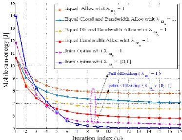
Mbits.

Figure 3. shows the value of the total energy consumption in the network according to algorithm iteration. As observed in Figure 3., when MUs use partial offloading to receive the service, the value of the energy consumption is lower than the other items.

Figure 4. shows the value of the total network energy consumption in terms of the upper bound of the acceptable MUs delay. As expected, the amount of energy consumption reduces with the increment of the delay upper bound. However, if the upper bound is very small, the value of energy consumption increases proportionately.

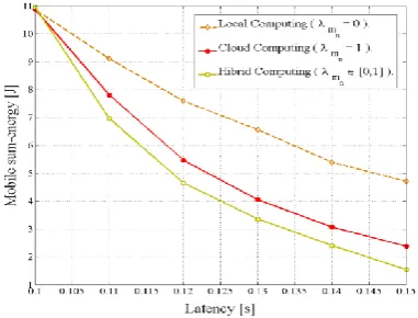
Figure 5. illustrates the total network energy consumption according to the upper bound of the acceptable MUs delay in three modes: local processing, cloud processing and joint processing (the combination of the cloud and local processing). As shown in Figure 5., by the joint allocation of resources in partial processing, the value of the total network energy consumption is significantly diminished compared to the local and cloud processing. For example, with max

0.15

n

m

 = sec, the value of the energy consumption is reduced to about 65% and 35% compared to the local processing and cloud processing, respectively.

(6)

Figure 4. Energy consumption versus the upper bound of the acceptable delay.

Figure 5. Comparison of total network energy consumption in the local, cloud and hybrid processing.

5. CONCLUSIONS

In this paper, we investigated the optimal allocation of the resources in a multi-cell network with MIMO. The

assigned resources were communication and

computational resources. The main goal of this model was to minimize the value of energy consumption with delay constraint. We expressed the problem of the resources optimal allocation in the form of the optimization problem in mathematical form. Since the problem was non-convex, we employed the SCA iterative algorithm for solving the problem. We assumed that the backhaul link capacity between BSs and CS was restricted and the MUs could send a part of the processing for computing. The simulation results showed that the jointly resources optimal allocation led to lower energy consumption. Also, the delay value was significantly reduced. Furthermore, the number of MUs was able to receive the service from CS, was increased.

6. REFERENCES

1. Jeyanthi, N., Shabeeb, H., Durai, M.S. and Thandeeswaran, R., "Rescue: Reputation-based service for cloud user environment",

International Journal of Engineering-Transactions B: Applications, Vol. 27, No. 8, (2014), 1179-1186.

2. Gubbi, J., Buyya, R., Marusic, S., Palaniswmi, M., "Internet of Things (IoT): A vision, architectural elements, and future directions", Future Generation Computer Systems, Vol. 29, No. 7, (2013), 1645-1660.

3. Palacin, M., "Recent advances in rechargeable battery materials: a chemists perspective", Chemical Society Reviews, Vol. 38, No. 9, (2009), 2565-2575.

4. Abolfazli, S., Sanaei, Z., Ahmed, E., Gani, A., Buyya, R., "Cloud-based augmentation for mobile devices: motivation, taxonomies, and open challenges", IEEE Communications Surveys & Tutorials, Vol. 16, No. 1, (2014), 337-368.

5. Fernando, N., Loke, S., Rahayu, W., "Mobile cloud computing: A survey", Future Generation Computer Systems, Vol. 29, No. 1, (2013), 84-106.

6. Liu, Yanchen, Myung, Lee., Zheng, Yanyan., "Adaptive multi-resource allocation for cloudlet-based mobile cloud computing system", IEEE Transactions on Mobile Computing, Vol. 15, No. 10,(2016), 2398-2410.

7. Song, Weiguang, Xiaolong, Su., "Review of mobile cloud computing", Communication Software and Networks (ICCSN), 2011 IEEE 3rd International Conference on.IEE, (2011), 1-4. 8. Satyanarayanan, M., et al, "The case for VM-based cloudlets in

mobile computing", IEEE pervasive Computing,(2009), 14-23. 9. Barbarossa, S., Sardellitti, S., Di Lorenzo, P., "Computation offloading for mobile cloud computing based on wide cross-layer optimization", in Proc. of Future Network and Mobile Summit

(FuNeMS2013), (2013), 1-10.

10. Barbarossa, Sardellitti, Di Lorenzo, "Joint allocation of computation and communication resources in multiuser mobile cloud computing", in Proc. of IEEE Workshop on Signal

Processing Advances in Wireless Communications (SPAWC2013), Darmstadt, Germany, (2013), 26-30.

11. Barbarossa, Sardellitti, Di Lorenzo, "Communicating while computing: Distributed mobile cloud computing over 5G heterogeneous networks", IEEE Signal Processing Magazine, Vol. 31, No. 6, (2014), 45-55.

12. Chen, X., "Decentralized computation offloading game for mobile cloud computing", IEEE Transactions on Parallel and

Distributed Systems, 2014.

13. Nouri, N., Rafiee, P., Tadaion, A., “NOMA-Based Energy-Delay Trade-Off for Mobile Edge Computation Offloading in 5G Networks", in 9th International Symposium on Telecommunications (IST) (2018), 522-527.

14. Sardellitti, Stefania, Scutari, G., Barbarossa, S., "Joint optimization of radio and computational resources for multicell mobile-edge computing", IEEE Transactions on Signal and Information Processing over Networks,No. 2, (2015), 89-103. 15. Zhang, W., Wen, Y., Guan, K., Dan, K., Luo, H., Wu, D., "Energy optimal mobile cloud computing under stochastic wireless channel", IEEE Transactions on Wireless Communications, Vol. 12, No. 9, ( 2013), 4569–4581.

(7)

Joint Allocation of Computational and Communication Resources to Improve Energy

Efficiency in Cellular Networks

N. Nouri, A. Entezari

Cell Lab, Department of Electrical Engineering, Yazd University, Yazd, Iran

P A P E R I N F O

Paper history:

Received 22 October 2018

Received in revised form 30 April 2019 Accepted 03 May 2019

Keywords:

Mobile Cloud Computing Heteregeneous Network Non-convex Function Bandwidth Allocation Convex Approximation

هدیکچ

هديکچ

–

نف کی لیابوم یربا شزادرپ روهظون یروآ

تیدودحم رب هبلغ یارب هک تسا یشوگ یاه

یاه ابوم ی ل ( ،یرتاب دننام

هريخذ تيفرظ ،یشزادرپ ناوت ،)هريغ و یزاس

فدهاب شزادرپ لماش( همانرب زا یشخب لاسرا )نيگنس تابساحم و هديچيپ یاه

حرطم یربا رورس تمس هب حرطم یجورخ دنچ و یدورو دنچ لماش یلولس دنچ متسيس ،هلاقم نیا رد .تسا هدش

تسا هدش

لولس نورد ناربراک هک ماجنا یارب اه

یم سیورس یاضاقت ،کرتشم یربا رورس زا دوخ شزادرپ هلأسم ،نينچمه .دننک

لخت هي

هب هنيهب هنيهب هلأسم کی تروص یم حرطم یزاس

هک دوش اهرتماراپ هنيهب ی عبانم لماش یزاس تارباخم

ی ( ناوت ،دناب یانهپ دننام

عبانم و )لاهکب کنيل تيفرظ و یلاسرا تابساحم

ی ( س یتابساحم تيفرظ دننام ريسم رد هکبش نورد )یربا رور

.دنتسه وسارف

یژرنا لک عومجم ،ربراک ره یارب ريخأت ديق تیاعر اب هک تسا نیا یلصا فده فرصم

هدش طسوت شزادرپ ماجنا یارب

یشور زا نآ لح یارب هک دش دهاوخ بدحمان هلأسم کی هب رجنم هلأسم نیا حرط .دوش لقادح هکبش ناربراک مانب

SCA

یم هدافتسا جیاتن .دوش هيبش زا لصاح ناشن یزاس

هنيهب هک تسا نیا هدنهد نازيم شهاک هب رجنم ،اهرتماراپ نیا مأوت یزاس

هکبش رد یژرنا فرصم یم

.دوش