Modeling overdispersed longitudinal binary data using a combined beta and normal random-effects model

M E T H O D O L O G Y

Open Access

Modeling overdispersed longitudinal binary data

using a combined beta and normal random-effects

model

Wondwosen Kassahun

, Thomas Neyens

, Geert Molenberghs

, Christel Faes

and Geert Verbeke

Abstract

Background:In medical and biomedical areas, binary and binomial outcomes are very common. Such data are often collected longitudinally from a given subject repeatedly overtime, which result in clustering of the

observations within subjects, leading to correlation, on the one hand. The repeated binary outcomes from a given subject, on the other hand, constitute a binomial outcome, where the prescribed mean-variance relationship is often violated, leading to the so-called overdispersion.

Methods:Two longitudinal binary data sets, collected in south western Ethiopia: the Jimma infant growth study, where the child’s early growth is studied, and the Jimma longitudinal family survey of youth where the adolescent’s school attendance is studied over time, are considered. A new model which combines both overdispersion, and correlation simultaneously, also known as the combined model is applied. In addition, the commonly used methods for binary and binomial data, such as the simple logistic, which accounts neither for the overdispersion nor the correlation, the beta-binomial model, and the logistic-normal model, which accommodate only for the overdispersion, and correlation, respectively, are also considered for comparison purpose. As an alternative estimation technique, a Bayesian implementation of the combined model is also presented.

Results:The combined model results in model improvement in fit, and hence the preferred one, based on likelihood comparison, and DIC criterion. Further, the two estimation approaches result in fairly similar parameter estimates and inferences in both of our case studies. Early initiation of breastfeeding has a protective effect against the risk of overweight in late infancy (p = 0.001), while proportion of overweight seems to be invariant among males and females overtime (p = 0.66). Gender is significantly associated with school attendance, where girls have a lower rate of attendance (p = 0.001) as compared to boys.

Conclusion:We applied a flexible modeling framework to analyze binary and binomial longitudinal data. Instead of accounting for overdispersion, and correlation separately, both can be accommodated simultaneously, by allowing two separate sets of the beta, and the normal random effects at once.

Keywords:Bernoulli model, Beta-binomial model, Binomial model, Logistic-normal model, Maximum likelihood

* Correspondence: [email protected] 2

I-BioStat, Center for Statistics, Universiteit Hasselt, Diepenbeek B-3590, Belgium

Full list of author information is available at the end of the article

Background

In medical and biomedical areas, binary and binomial out-comes are very common. The generalized linear model family [1-3] offers, among others, a suitable modeling framework. Such data are often collected repeatedly in time. Letrijbe a longitudinal binary outcome for subject i

at thejthtime point, such that each subject hasni

measure-ments. The sum Yi¼

Pni

j¼1rij follows a binomial distribu-tion. It is well known that, while i.i.d. Bernoulli variables do not contradict the prescribed mean-variance relation, i.i.d. binomial data can, exhibiting extra variability beyond the binomial model, leading to the so-called overdispersion in the latter, in addition to the correlation emanating from the repeated measures nature. In the past, overdispersion and correlation have been handled separately. To deal with overdispersion, the beta-binomial model is a popular and analytically tractable alternative to the binomial model, which accounts for the overdispersion not accommodated for in the binomial model, thereby allowing for a better fit to the observed data [4,5]. On the other hand, correlation is accommodated for by making use of generalized linear mixed models [6-8], which combine the general exponen-tial family models with normally distributed random effects, are attractive for repeated measurements. In this paper, we use a general and flexible framework for such combina-tions, proposed by Molenberghs et al [9]. These authors focused on likelihood based methods for inference. In this paper, we have tried to present how the new combined model proposed by Molenberghs et al [9], can be imple-mented in the Bayesian paradigm. In addition, the ability to specify prior distribution will help to incorporate more in-formation in inference, especially for complex models, like the combined model, that attempt to capture overdisper-sion and clustering using two separate sets of random effects. Further, we considered two real world data sets and analyzed, first in the likelihood context, and then in the Bayesian, which could also be considered as sensitivity analysis.

Two longitudinal binary data sets, collected in south western Ethiopia: the Jimma infant growth study, where the child’s early growth is studied, and the Jimma longi-tudinal family survey of youth where the adolescent’s school attendance is studied over time, are considered. One of the key indicators of infant growth is Body Mass Index (BMI). Many studies suggest that Breastfeeding status, and socio-economic condition of the parents, among others, are potential risk factors of BMI [10-12]. School attendance among adolescents varies among gen-der groups in a way that girls are at higher risk of school absenteeism as compared to boys. Moreover, adolescents living in urban areas have have a better school attend-ance rate, unlike those in the rural setting [13,14].

The paper is organized as follows. Section (Methods) briefly reviews standard methods and presents the model combining the normal and conjugate random effects in Section (Models combining conjugate and normal random effects). Avenues for parameter estimation and ensuing inferences are explored in Section (Estimation), with particular emphasis on so-called partial marginalization and Bayesian estimation. The results for the analysis are presented in Section (Results) followed by discussed in Section (Discussion). Some concluding remarks are taken up in Section (Conclusion).

Methods

In this section, we preset the two data sets from the Jimma case studies and briefly describe conventional models used for analysis. We start this section with pre-senting the data followed by a review of the generalized linear model; we also lay out the notation for the rest of the paper. Section (Overdispersion models) focuses on overdispersion in the binary and binomial situations. Section (Models with normal random effects) reviews the mixed model methodology for longitudinal data ana-lysis. Finally, in Section (Models combining conjugate and normal random effects), the combined model is pre-sented in which ideas from the mixed model method-ology are combined with ideas on overdispersion.

The Jimma case studies

Two longitudinal datasets, Jimma Infant Growth Study and Jimma Longitudinal Family Survey of Youth, collected in Southwest Ethiopia are considered.

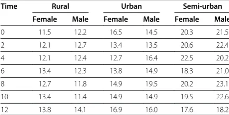
percentile for age- and sex-specific BMI classification of overweight is used based on Center for Disease Control (CDC) recommendation [16]. The question of interest is whether the percentage of overweight infants changes over time, and whether the evolution differs for gender, place of residence (rural, urban and semi-urban), as well as breast feeding behavior. Table 1 gives a summary of the percen-tage of overweight infants as a function of gender, location and follow-up time (age).

The Jimma Longitudinal Family Survey of Youth (JLFSY) is another Ethiopian study where data were collected from households. The study began in 2005, and was repeated in 2007. More than 90% of the study subjects present at baseline were visited and willing to respond in the second round. The study population is representative of the relatively large town of Jimma, the small towns of Yebu, Serbo, and Sheki, and nearby rural areas. The sample includes 3700 households as well as 700 adolescents. In this paper, the outcome of interest is the adolescents’ current school attendance coded as 0 (not currently attending) or 1 (currently attending). Current school attendance was 90.2% and 91.1% in the first round survey and 93.5% and 92.8% in the second round for male and 3 female adolescents, respectively. The research question is to examine whether or not the percentage of school attendance depends on adolescents involvement in work to support themselves or their fa-milies to earn money, whether they are living in urban towns or rural areas, as well as on gender and age.

Standard generalized linear model

A random variable Y follows an exponential family distri-bution if the density is of the form

f yð Þ f y jη;ϕÞ ¼ expϕ1½yηψ ηð Þ þc yð ;ϕÞ;

ð1Þ

for a specific set of unknown parameters η and ϕ, and for known functions ψ() and c(, ). Often, ηand ϕ are

termed ‘natural parameter’ (or ‘canonical parameter’) and ‘dispersion parameter,’ respectively. For this family, in general, the mean and variance are related [17].

For binary responses, the model of interest is: Y Ber-noulli (π). We want to explain variability between outcome values based on covariate values with density function

f yð jη;ϕÞ ¼πyð1πÞ1y ¼ exp yln π

1π

þ ln 1ð πÞ

h i

: ð2Þ

The mean is given byμ=π and the variance, var (μ) = π(1−π) [1].

When collecting a set of data, letY1,. . .,YNbe a set of

independent binary outcomes, and let x1,. . ., xN

repre-sent the corresponding p-dimensional vectors of covari-ate values. With a logit link function, ln πi

1πi

¼x′iξ is the logistic regression model with ξ a vector of p fixed, unknown regression coefficients.

Overdispersion models

The standard Bernoulli model assumes that the mean and variance depend on a single parameter. Though a set of i.i.d. Bernoulli data cannot contradict the mean-variance re-lationship, it may not hold true for data having a hierarchical structure of the formzisuccesses out ofnitrials.

For the Jimma infants study, considering i.i.d. Bernoulli data, the sample average probability of success and the sample variance are 0.150 and 0.128, respectively, indicating that the prescribed mean-variance link is maintained. In contrast, in the binomial setting, taking the hierarchical structure into account, the sample average and the sample variances are 0.141 and 2.107, respectively implying that the sample contradicts the mean-variance relationship for these data.

Similar exploratory analyses on the Jimma Longitudinal Family Survey of Youth were undertaken. For the binomial response, taking the two repeated measurements results in sample average probability of success 0.919 and sample variance 0.168 indicating that the results are in line with the prescribed mean-variance relationship which is known to be always true for the Bernoulli case. This may suggest, at first sight, that these data are not prone to exhibit strong overdispersion, even in the hierarchical binomial setting. In addition to the exploratory analysis, we also made tests for overdispersion. The commonly use approach is to compute the ratio of the residual deviance to the residual degrees of freedom which is approximates the overdispersion para-meter (ϕ^). When the ratio is appreciably larger than 1, overdispersion is said to occur. It is pointed out that this approach could be misleading whennipiis not sufficiently

large, where pi is probability of the success event. This is

because it is based on asymptotic theory. As a result, a better approach is based on a quasi-binomial model which Table 1 Jimma Infant Growth Study

Time Rural Urban Semi-urban

Female Male Female Male Female Male

0 11.5 12.2 16.5 14.5 20.3 21.5

2 12.1 12.7 13.4 13.5 20.6 22.4

4 12.1 12.4 12.7 16.4 22.5 20.2

6 13.4 12.3 13.8 14.9 18.3 21.0

8 12.7 11.8 14.9 19.5 20.2 23.1

10 13.4 11.4 14.9 14.9 19.5 22.6

12 13.8 14.1 16.9 16.0 17.6 18.2

allows more dispersion than the binomial model [18]. The approximated overdispersion (ϕ^ = 2.37) computed as the ratio of the residual deviance to the residual degrees of free-dom in the Binomial, and the one estimated in the quasi-binomial model (ϕ^=2.47) for the Jimma Infants Growth data are very similar, both suggesting the presence of strong overdispersion. However, similar analysis for the Jimma Family Survey data does not suggest a considerable over-dispersion, with values 0.765 and 1.129, approximated by the ratio of the residual deviance to the residual degrees of freedom in the Binomial, and estimated by the quasi-binomial, respectively.

An elegant way to account for overdispersion is through the so-called beta-binomial model, in which the Bernoulli model is combined with a beta distribution [17,19].

Models with normal random effects

For non-Gaussian data, the well-known generalized linear mixed model, in which the linear predictor con-tains random effects in addition to the usual fixed effects, is a common choice [6-8]. These random effects are usually assumed to come from a normal distribution. The model can be specified as follows:

Let Yij be the jth outcome measured for subject

i= 1,. . ., N ,j= 1,. . ., ni and group the ni measurements

into a vector Yi. Assume that, in analogy with Section

(Standard generalized linear model), conditionally upon q- dimensional random effects b_iN (0, D), the out-comesYijare independent with densities of the form

fi yijjbi;ξ;ϕÞ ¼ exp ϕ1 yijλijψ λij þc yij;ϕ

;

ð3Þ with

η ψ′ _λ ij

¼η μij ¼η E Yijjbi;ξÞ

¼x′ijξþz′ijbi;

ð4Þ

for a known link function η(), with xij and zij p

-di-mensional and q-di-di-mensional vectors of known cov-ariate values, with ξ a p-dimensional vector of unknown fixed regression coefficients, and with ϕ a scale (overdispersion) parameter. Finally, let f (bi|D)

be the density of the N (0, D) distribution for the random effects bi.

Here, the hierarchical approach is needed because we are working with longitudinal data. More pre-cisely, in our model, the natural parameter is written as a linear predictor, a function of both fixed and random effects.

Models combining conjugate and normal random effects Combining both the overdispersion effects (Section Overdispersion models) and the normal random effects

(Section Models with normal random effects) into the generalized linear model framework, produces the fol-lowing general family [9]:

fi yijbi;ξ;θij;ϕ

¼ exp ϕ1 _y

ijλijψ λij

þc yij;ϕ

;

ð5Þ

with notation similar to the one used in (3), but now with conditional mean

E Yijbi;ξ;θij

¼μc

ij¼θijκij;

ð6Þ

where the random variable θij Gij (ϑij, σij), κij=g (xij′

ξ+zij′bi),ϑijis the mean ofθijandσijis the

correspond-ing variance. Finally, as before,biN (0, D). Writeηij= xij′ ξ+zij′ bi. Unlike in Section (Models with normal

random effects), we now have two different notations,ηij

and λij , to refer to the linear predictor and/or the

nat-ural parameter. The reason is that λij encompasses the

random variables θij , whereas ηij refers to the ‘GLMM

part’ only. A detailed overview of the model can be found in Molenberghs et al [9].

For the case of binary data, we assume that

yijBernoulli πij¼θijκij

; ð7Þ

κij¼

exp x′ijξþz′ijbi

1þ exp x′ijξþz′ijbi

; ð8Þ

whereθijBeta(α, β). Indeed, this model also intuitively

seems useful, as overdispersion and correlation due to the data hierarchy can occur simultaneously.

The model is a two-level model with two types of ran-dom effects: (a) the bi, to accommodate correlation

among repeated measures (and some overdispersion); (b) the θij for additional overdispersion. While (a) turns

the model into a two-level model, rather than a one-level one, (b) does not further add a one-level, because it merely accommodates overdispersion. This is to be com-pared with a classical generalized linear model, where also overdispersion random effects can be taken into ac-count (e.g., beta in the Bernoulli model to yield the beta-binomial; gamma in the Poisson model to yield the negative binomial; etc.), while keeping the so-resulting models remain one-level models.

Further, because the θij follow a conjugate

Estimation

In the likelihood framework, estimation proceeds by in-tegration. The likelihood contribution of subjectiis

fiðyijϑ;D;ϑi;ΣiÞ ¼Z Yni

j¼1

fij yijjϑ;bi;θiÞf bð ij ÞDfðθijϑiΣiÞdbidθi:

ð9Þ From this, the likelihood is given as:

Lðϑ;D;ϑ;ΣÞ ¼Y

N

i¼1

fiðyijϑ;D;ϑi;ΣiÞj

¼YN i¼1

Z Yn

ð10Þ Here,ϑgroups all parameters in the conditional model forYi. In the binomial case, the expression takes the form:

f zijjnij;bi

¼ X

nijzij

t0

1 ð Þt

κzijþt

ij

nij! zij!t! nijzijt

!

B zijþtþαj;βj

B αj;βj

ð11Þ with

κij¼

exp x′ijξþz′ijbi

1þ exp x′ijξþz′ijbi

It is straightforward to obtain the fully marginalized probability by numerically integrating over the normal random effects, and using a tool such as the SAS pro-cedure NLMIXED that allows for normal random effects in arbitrary, user-specified models. More details can be found in [9].

As an alternative estimation method, we turn to the Bayesian paradigm, combined with the popular Markov Chain Monte Carlo (MCMC) technique, making analyses of real-world complex data feasible [15]. In the Bayesian ap-proach, prior distributions are assigned to the parameters and the random effects to adjust for parameter uncertainty. Bayesian inference for estimation of parameterθ is based on the posterior distribution, which is proportional to the likelihood multiplied with the prior distribution.

The Jimma longitudinal studies are characterized by clustering, resulting form the repeated measurements, leading to both correlation and overdispersion. When mo-deling such data, incorporating prior distribution for model parameters, including that of subject and observation spe-cific random effects, will better handle the underlying uncertainties, instead of assuming that they are fixed. With

the same model specification as in the likelihood frame-work, the parametersξ, bi, andθijare taken to be a priori

independent, i.e.,p(ϑ, D,ϑi,Σi) =p(ϑ)p(D)p(ϑi)p(Σi) and the

following prior distributions are used:

ξN(0,10−6), biN(0,τi), as also suggested in the

lit-erature [15,16], andθijBeta(α,β), is unimodal and

con-cave, whenα>1,β>1 [3]. For the hyper parametersτi,

the inverse-Gaussian prior IG(0.001, 0.001), and for α and β, an improper uniform prior is used, as also sug-gested by Gelman et al [16]. For more information on Bayesian data analysis and MCMC methods see [20,21].

Note that the Beta-binomial distribution is a com-pound distribution of the binomial and its conjugate beta, which can be used to capture overdispersion in bi-nomial data. Beta-bibi-nomial approximates the bibi-nomial distribution arbitrarily well when its two non-negative parameters, α and β, determining its shape, are suffi-ciently larger. If one or both of these parameters are less than 1, then the probability mass function will go to in-finity near its boundaries, 0 and 1, and hence not con-cave. As a result, the mode does not exist, leading to computational problems in MCMC. For this reason, we used the restrictionα>1,β>1, such that the density is always concave and unimodal whereby it is always finite over the support [0, 1].

Spiegelhalter et al [22] suggest to use the so-called De-viance Information Criterion for model com- parison in Bayesian inference. Assume a probability model P (y|θ). The effective number of param- eters with respect to a model with parameterΘis given bypD{y,Θ, ~θ(y)} = E_θ|y

[−2 log p(y|θ)] + 2 log[p{y|θ(y)}]. We shall usually drop the arguments {y, Θ, ~θ(y)} from notation. Generally, we take θ~(y) =E(θ|y), the posterior mean of the parameters. For f (y) being a fully specified standardizing term that is a function of the data alone, pD, defined as a‘mean devi-ance minus the devidevi-ance of the means,’is given bypD=

E[D(θ|y)]−D(E[θ|y]), whereD(θ) =−2 logP(y|θ) + 2 log

f (y) is the Bayesian deviance, used as a measure for goodness of fit. The deviance information criterion (DIC), defined as the classical estimate of fit plus twice the effective number of parameters DIC =D(E[θ|

based on DIC, the important risk factors could be identi-fied looking the credible intervals, considering whether zero is in or outside of the credible interval.

We also attempted to fit the beta-binomial marginal density, although it is not one commonly encountered in software packages like WinBugs, where an observation xi contributes a likelihood term Li. We used the

so-called zero trick, a Poi(ϕ) observation of zero has likeli-hood exp(−ϕ), so if our observed data is a set of 0’s, and ϕi is set to−log(Li), we would obtain the correct

likeli-hood contribution [23]. This zero trick allows for arbi-trary sampling distributions and is particularly suitable when, say, dealing with truncated distributions. However, our case studies showed that this method can be very in-efficient and give a very high Monte Carlo error.

In terms of parameter interpretation, we would like to refer back to the beneficial properties that come with the conjugacy property. Indeed, because the θij follow a

conjugate distribution, the interpretation of the para-meters is the same as in a classical generalized linear mixed model. Precisely, this means that the effect on the regression parameters only comes from the normal ran-dom effects in the linear predictor, a fact well documen-ted. For a review, see, for example, Molenberghs and Verbeke [17].

Results

The jimma infant growth study

We will analyze the binary BMI data. The following model is assumed for the mean structure:

Yij|biBernoulli(πij), for subjectiand measurementj,

and

logit πij ¼ξ0þb0iþðb1iþξ1ÞTijþξ2Giþξ3P1i þξ4P2iþξ5Bij

¼ξ6GiTijþξ7P1iTijþξ8P2iTijþξ9BijTij; ð12Þ

where Gi is a gender indicator, P1i and P2i are dummy

variables for place of residence corresponding to rural and urban areas and using semi-urban areas as a refer-ence.Tij is the time point at which thejth measurement

is taken for the ith subject, which is centered at month six.Bijdenotes whether theithinfant is breast fed or not

at timej. The random interceptbiN(0,D).

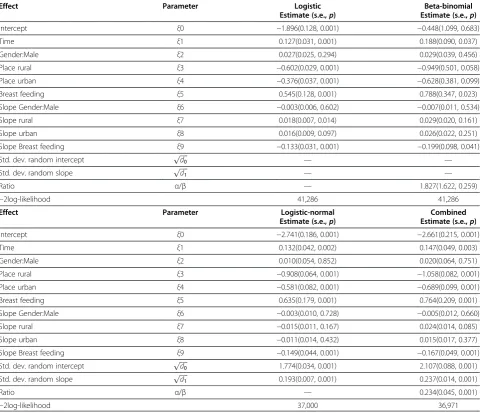
The Infant Growth dataset is analyzed with a simple logistic model, a beta-binomial model introducing only an overdispersion parameter, a random-effects logistic model that introduces a random-effects term to take the repeated structure of the data into account, and finally the combined model, which allows for both an overdis-persion and a random effects term. Parameter estimates are presented in Table 2.

Clearly, the logistic-normal model is an important im-provement, in terms of likelihood, relative to both the ordinary logistic model and the beta-binomial. Moreover, considering the combined model, there is a very strong improvement in fit when the beta and normal random effects are simultaneously allowed for. The overdispesion term in the combined model is significant (p<0.001), implying the presence of considerable extra variability due to the grouped nature of the data, which is beyond what can be accommodated by the commonly used logistic-normal model.

The logistic-normal model ignores the overdispersion that results from the grouped nature of the data. On the other hand, the beta-binomial model accommodates overdispersion which is assumed independent, implying independence between repeated measurements. Again, this is not realistic and therefore the combined model is the more viable candidate, supported further by the aforementioned 9 likelihood comparison.

The combined suggests that the intercept, the time ef-fect, main effects of place of residence and breastfeeding are significant, which is also true for time interaction with rural place of residence and breast feeding. How-ever, main effect and slope of gender were not significant implying that proportion of overweight seems to be in-variant among male and female infants over time. Infants living in rural, and urban areas are at lower risk of overweight as compared to those in semi-urban ares with (ξ3=−1.058, p = 0.001), and (ξ4=−0.689, p = 0.001),

respectively. Further, early initiation of breastfeeding has a protective effect against the risk of overweight in late infancy (ξ9=−0.167, p = 0.001), as shown in Table 2.

Jimma longitudinal family survey of youth

We will now analyze current school attendance. For the logit, consider the model: Yij|biBernoulli(πij), with

logit πij ¼ξ0þbiþξ1Aijþξ2Giþξ3P1ij

þξ4P2ijþξ5Wijþξ6Rij; ð13Þ

whereAijis the age of theithsubject at thejthvisit, Giis the

gender of the ith subject. P1ij and P2ij denote the two

dummy variables for place of residence of theithsubject on the jth visit, which are urban, semi-urban, and rural by taking rural as a reference. Wij indicates whether the ith

adolescent is engaged in some work for the family or help support on thejthvisit. Finally,Rijis thejthround or

mea-surement occasion of theithsubject, andbiN(0,d).

comparisons of the simple logistic and the beta-binomial on the one hand, as well as the logistic-normal and the combined, on the other. One can easily see, however, that the commonly used logistic-normal and the com-bined models are significant improvements over the standard logistic model. We further observe, while the logistic- normal model suggests a significant intercept (p = 0.045), that the same does not emerge when the combined model is considered (p = 0.099) implying the beta random effect still has some impact on the p-values. The logistic- normal model is adequate, in this case study, for the combined model where there is no strong evidence of overdispersion, as the overdispersion term is not significant (p = 0.29)for these data with two repeated measurements per subject, as mentioned in the earlier

sections. Further extension by adding random slope did not improve the fit of both logistic-normal and the com-bined models (details not shown).

Adolescents living in urban, and semi-urban areas have higher school attendance than those living in rural areas, with (ξ2= 1.098, p = 0.001), and (ξ3= 1.092,

p = 0.001), respectively. Gender is also significantly asso-ciated with school attendance, where female adolescents are lower (ξ4=−1.241, p = 0.001). There is evidence that

school attendance increases in the second round visit than that of the first (ξ6= 0.398, p = 0.010).

Comparison between estimation methods

For comparison with the previously applied estimation method in the likelihood framework, we again apply the Table 2 Jimma Infant Growth Study

Effect Parameter Logistic Beta-binomial

Estimate (s.e.,p) Estimate (s.e.,p)

Intercept ξ0 −1.896(0.128, 0.001) −0.448(1.099, 0.683)

Time ξ1 0.127(0.031, 0.001) 0.188(0.090, 0.037)

Gender:Male ξ2 0.027(0.025, 0.294) 0.029(0.039, 0.456)

Place rural _ξ3 ₋0.602(0.029, 0.001) ₋0.949(0.501, 0.058)

Place urban ξ4 −0.376(0.037, 0.001) −0.628(0.381, 0.099)

Breast feeding ξ5 0.545(0.128, 0.001) 0.788(0.347, 0.023)

Slope Gender:Male ξ6 −0.003(0.006, 0.602) −0.007(0.011, 0.534)

Slope rural ξ7 0.018(0.007, 0.014) 0.029(0.020, 0.161)

Slope urban ξ8 0.016(0.009, 0.097) 0.026(0.022, 0.251)

Slope Breast feeding ξ9 −0.133(0.031, 0.001) −0.199(0.098, 0.041)

Std. dev. random intercept ffiffiffiffiffid0

p

— —

Std. dev. random slope pffiffiffiffiffid1 — —

Ratio α/β — 1.827(1.622, 0.259)

−2log-likelihood 41,286 41,286

Effect Parameter Logistic-normal Combined

Estimate (s.e.,p) Estimate (s.e.,p)

Intercept ξ0 −2.741(0.186, 0.001) −2.661(0.215, 0.001)

Time ξ1 0.132(0.042, 0.002) 0.147(0.049, 0.003)

Gender:Male ξ2 0.010(0.054, 0.852) 0.020(0.064, 0.751)

Place rural ξ3 −0.908(0.064, 0.001) −1.058(0.082, 0.001)

Place urban _ξ4 ₋0.581(0.082, 0.001) ₋0.689(0.099, 0.001)

Breast feeding ξ5 0.635(0.179, 0.001) 0.764(0.209, 0.001)

Slope Gender:Male ξ6 −0.003(0.010, 0.728) −0.005(0.012, 0.660)

Slope rural ξ7 −0.015(0.011, 0.167) 0.024(0.014, 0.085)

Slope urban ξ8 −0.011(0.014, 0.432) 0.015(0.017, 0.377)

Slope Breast feeding ξ9 −0.149(0.044, 0.001) −0.167(0.049, 0.001)

Std. dev. random intercept pffiffiffiffiffid0 1.774(0.034, 0.001) 2.107(0.088, 0.001)

Std. dev. random slope ffiffiffiffiffid1

p

0.193(0.007, 0.001) 0.237(0.014, 0.001)

Ratio α/β — 0.234(0.045, 0.001)

−2log-likelihood 37,000 36,971

same models to the two surveys, but now in the Bayesian framework. After generating 70,000 MCMC samples for the combined, and 50,000 MCMC samples for logistic-normal, beta- binomial, and simple logistic, the first 10,000 samples are discarded and treated as so-called burn-in samples. The remaining samples are used to summarize the posterior estimates. Two distinct chains were used to check sensitivity to the initial values, and convergence was met. Convergence was checked using the Gelman-Rubin diag-nostic as well as by visual inspection of the trace and QQ plots [24].

The posterior summaries of logistic, beta-binomial, logistic-normal, and combined models are given in Tables 4 and 5 for the Jimma Infants Growth dataset and the Jimma Longitudinal Family Survey of Youth, re-spectively. The parameter estimates are fairly similar with what was obtained previously in the likelihood ap-proach in both cases, except for differences in the case of the beta-binomial for the Jimma Infants data in Table 4 when compared with Table 2.

In terms of significance of the parameters, the same con-clusion is reached for the two case studies in both

approaches, except that the beta-binomial for the intercept and time effects in Jimma infants study shows significance in the likelihood framework as given in Section (The jimma infant growth study), while the same does not emerge from the Bayesian case, as observed from the 95% credible inte-val which include zero for these effects. We compared the various models using the DIC criterion. For both studies, there is a significant reduction in the DIC of the logistic-normal and the beta-binomial, as compared to the simple logistic. We observe a rather high degree of model im-provement by combining beta and normal random effects simultaneously, to allow for both the overdispersion and the data hierarchy. Moreover, the logistic and the beta-binomial ignore the correlation stemming from the data hierarchy on the one hand, and the logistic-normal does not allow for the overdispersion, on the other, which altogether make the combined model the preferred one.

According to Spiegelhalter et al [22], in comparing complex hierarchical models where the number of para-meters are not clearly defined, pD is the difference be-tween the posterior mean of the deviance and the deviance at the posterior means of the parameters of Table 3 Jimma Longitudinal Family Survey of Youth

Effect Parameter Logistic Beta-binomial

Estimate (s.e.,p) Estimate (s.e.,p)

Intercept ξ0 1.171(0.626, 0.061) 1.155(0.702, 0.099)

Age ξ1 0.039(0.049, 0.414) 0.044(0.055, 0.421)

Place urban ξ2 0.971(0.148, 0.001) 1.089(0.266, 0.001)

Place semi-urban _ξ3 0.979(0.159, 0.001) 1.104(0.284, 0.001)

Gender:Female ξ4 −1.111(0.123, 0.001) −1.226(0.237, 0.001)

Work ξ5 0.134(0.122, 0.274) 0.146(0.138, 0.288)

Round ξ6 0.341(0.141, 0.016) 0.390(0.178, 0.029)

Std. dev. random effect pffiffiffid — —

Ratio α/β — 0.009(0.014, 0.528)

−2log-likelihood 1987.7 1987.4

Effect Parameter Logistic-normal Combined

Estimate (s.e.,p) Estimate (s.e.,p)

Intercept ξ0 1.443(0.719, 0.045) 1.463(0.888, 0.099)

Age _ξ1 0.046(0.056, 0.408) 0.058(0.070, 0.408)

Place urban ξ2 1.098(0.178, 0.001) 1.379(0.393, 0.001)

Place semi-urban ξ3 1.092(0.189, 0.001) 1.339(0.368, 0.001)

Gender:Female ξ4 −1.241(0.147, 0.001) −1.499(0.339, 0.001)

Work ξ5 0.153(0.144, 0.287) 0.189(0.182, 0.296)

Round ξ6 0.398(0.155, 0.010) 0.519(0.237, 0.028)

Std. dev. random effect pffiffiffid 1.138(0.188, 0.001) 1.342(0.318, 0.001)

Ratio _α/_{β —} 0.013(0.013, 0.293)

−2log-likelihood 1972.9 1972.1

Parameter estimates, standard errors, and p-values for the regression coefficients in (1) the logistic model, (2) the beta-binomial model, (3) the logistic-normal model, and (4) the combined model.

interest, not only measures the effective number of para-meters but also the model complexity. These authors further noted that the contribution pDiof each

observa-tion i turned out its leverage, defined as the relative in-fluence that each observation has on its own fitted value. for yi conditionally independent given θ, pDi, shows its

interpretation as the difficulty in estimating θ with yi.

This shows the connection between the sample size, the parameters to be estimated, and the pD. The Jimma infants (n = 7969) and the Jimma Longitudinal family survey (n = 2100) data have large number of subjects followed longitudinally, where each subject was mea-sured seven and two times, respectively. Due to these

reasons, the pD values, as presented in Tables 4 and 5, appeared to be larger as the by-product of the MCMC estimation to obtain leverage of each observation.

Unlike the Jimma infants study in Table 4, pD of the combined model for the Jimma Longitudinal Family Survey of Youth in Table 5, (pD= 211.9), is lower than that of the logistic-normal (pD= 241.5). This implies that, for the Jimma Longitudinal Family Survey of Youth, the combined model is less complex to fit than the logistic-normal, al-though, this is what we don’t usually expect, as the com-bined model seems more complex, since it includes both the beta and the normal random effects, while, the logistic-normal including only the normal random-effects. Table 4 Jimma Infant Growth Study

Effect Logistic Beta-binomial

Mean(s.d.) Mean(s.d.)

Intercept ξ0 −1.894(0.123) −1.486(1.488)

Time ξ1 0.126(0.031) 0.155(0.207)

Gender:Male ξ2 0.027(0.026) 0.003(0.066)

Place rural _ξ3 ₋0.602(0.029) ₋2.486(1.290)

Place urban ξ4 −0.377(0.037) −1.973(1.210)

Breast feeding ξ5 0.543(0.123) 1.126(0.294)

Slope Gender:Male ξ6 −0.003(0.006) −0.015(0.016)

Slope rural ξ7 0.018(0.007) 0.160(0.178)

Slope urban ξ8 0.015(0.009) 0.1610.182)

Slope Breast feeding ξ9 −0.132(0.030) −0.289(0.097)

Std. dev. random intercept ffiffiffiffiffid0

p

— —

Std. dev. random slope pffiffiffiffiffid1 — —

Ratio α/β — 3.222(0.524)

DIC 41,310.0 40,390.0

pD 9.9 2511.0

Effect Logistic-normal Combined

Mean(s.d.) Mean(s.d.)

Intercept ξ0 −2.773(0.191) −2.755(0.258)

Time ξ1 0.137(0.042) 0.169(0.062)

Gender:Male ξ2 0.020(0.054) 0.026(0.069)

Place rural _ξ3 −0.915(0.065) −1.115(0.085)

Place urban ξ4 −0.606(0.083) −0.749(0.103)

Breastfeeding ξ5 0.666(0.185) 0.903(0.253)

Slope Gender:Male ξ6 −0.003(0.010) −0.006(0.012)

Slope rural ξ7 0.015(0.011) 0.026(0.015)

Slope urban ξ8 0.011(0.014) 0.017(0.018)

Slope Breastfeeding ξ9 −0.144(0.041) −0.192(0.061)

Std. dev. random intercept ffiffiffiffiffid0

p

1.783(0.035) 2.212(0.074)

Std. dev. random slope ffiffiffiffiffid1

p

0.193(0.007) 0.250(0.013)

Ratio α/β — 0.288(0.031)

DIC 33,605.1 33,377.6

pD 5400.7 6218.3

However, for these specific data, this resulted likely because there is less conflict between the specific data set, and the prior distributions which could be associated to the conju-gacy of the beta random effects, as well as the peculiar data features including number of subjects and repeated mea-surements per subject.

The SAS and WinBugs codes used for analysis of the data sets are given in the Appendix.

Discussion

Analysis of the case studies show that, in the presence of overdispersion, and clustering, the combined model results in improvement in model fit, which is similar to the finding in Molenberghs et al [9].

This study revealed that early breastfeeding lowers the risk of overweight at late infancy. This finding is in line with Bergman et al [10], who showed that breastfed infants had lower BMI after 3 months from birth than bottle-fed infants, though the BMIs at birth were nearly identical in both groups. Owen et al [11], who reviewed sixty-one studies, states that initial breastfeeding

protects against obesity in later life, although the precise magnitude of the association remains unclear. Unlike Owen et al [11], the present study showed that, infants in the breastfed group were fatter, at birth, as compared to those who were not breastfed. This is likely because of the unmeasured maternal history, such as maternal BMI, and socio-cultural aspects, which are considered to be the risk factors of overweight in children [25]. In addition, it is a common practice in the study area that mothers provide additional liquid or solid food starting from early infancy, in addition to breastfeeding. This is probably because they believe that a child with more weight is considered as healthy, which is likely to have its own impact on the BMI in the early infancy. In this study, it is also shown that place of residence does not have a long term effect in the risk of overweight, instead it is the mode of feeding which is more important. The baseline dif-ferences observed in the risk of overweight among infants living in urban, semi-urban areas might be attributable to other family related factors like, social class, family income, educational level of the parents, and other socio-cultural variables, which are indicated to affect the nutrition of young children and women in Ethiopia [12].

In investigating school attendance among adolescents, this study showed that, girls have a lower rate of current school attendance than boys, which is a common situ-ation in most Sub-Saharan African Countries. According to World Health Organization [13], there is a clear gen-der gap observed in primary or secondary school enroll-ment when the Gender Parity Index (GPI), the ratio of female to male enrollment, is considered. Between the years 1999 and 2003, GPI was found to be 0.7, indicating that there were only 7 girls enrolled at primary schools for every 10 boys. This gender gap increases with in-creasing level of education. This study also showed that adolescents in urban and semi-urban areas have higher rate of than those in the rural areas, which is in line with report of World Bank [14], where it was stated that among children in rural areas with a school in the neigh-borhood, less than 44% registered for school; in urban areas, the percentage is much higher up to 86%. Accord-ing to the report, distance to the nearest school, house-hold characteristics, and learning environment were among the possible reasons of the gap in the school attendance.

Conclusion

We have presented a model which integrates normal and beta random effects into a single model, termed the com-bined model. Our work builds upon that of Molenberghs et al [9], who brought together normal random effects to in-duce association between repeated binary and binomial data, and a beta-binomial distributed random factor in the log-linear predictor to fine tune the overdispersion.

Table 5 Jimma Longitudinal Family Survey of Youth

Effect Logistic Beta-binomial

Mean(s.d.) Mean(s.d.)

Intercept ξ0 1.185(0.624) 1.151(0.731)

Age ξ1 0.039(0.049) 0.047(0.057)

Place urban ξ2 0.977(0.148) 1.134(0.183)

Place semi-urban _ξ3 0.987(0.161) 1.161(0.202)

Gender:Female ξ4 −1.113(0.123) −1.266(0.148)

Work ξ5 0.133(0.122) 0.154(0.140)

Round ξ6 0.343(0.142) 0.404(0.165)

Std. dev. random effect pffiffiffid — —

Ratio α/β — 0.0111(0.0029)

DIC 2002.0 2001.0

pD 6.97 13.77

Effect Logistic-normal Combined

Mean(s.d.) Mean(s.d.)

Intercept _ξ0 1.452(0.732) 1.272(0.953)

Age ξ1 0.047(0.057) 0.077(0.078)

Place urban ξ2 1.107(0.180) 1.427(0.270)

Place semi-urban ξ3 1.104(0.192) 1.382(0.269)

Gender:Female ξ4 −1.247(0.149) −1.528(0.214)

Work ξ5 0.155(0.145) 0.199(0.184)

Round ξ6 0.401(0.157) 0.521(0.203)

Std. dev. random effect pffiffiffid 1.148(0.203) 1.417(0.266)

Ratio α/β — 0.013(0.003)

DIC 1943.0 1915.0

pD 241.5 211.9

Maximum likelihood estimation was considered by in-tegrating over the random effects using the SAS proced-ure NLMIXED.

Further, Bayesian inference has been applied. Prior in-formation about the parameters induces correlation, which then leads to reduced effective dimensionality al-though the reduction depends on the available data [22]. Complexity reflects the difficulty in fit and hence it seems reasonable that the measure of complexity may depend on both the prior information concerning the parameters under scrutiny and the specific data that are observed. This can be elucidated from the Jimma Longi-tudinal Family Survey of Youth result, where the com-bined model is less complex in fit, which likely results from the conjugacy of the beta random effect and the number of subjects as well as the repeated measure-ments per subject.

Future studies on early growth of children could bene-fit from careful measurement of a wider range of poten-tial confounders of overweight.

Further efforts should be made to fill the gap in school attendance among boys and girls, as well as, urban and rural areas by focusing on the potential causes, such as lagging experience in primary schooling, which is then exacerbated by such factors as the practice of early mar-riage among Ethiopian women, families reluctance to in-vest in girls education. Situating schools closer to childrens homes in rural areas, and improve the quality of the services is necessary [14]. Longitudinal studies with better number of repeated measurements per sub-ject should be conducted to get better insight on the trends of school enrollment, survival of adolescents.

Appendix

SAS Implementation

This section shows a SAS program, using the procedure NLMIXED, for the combined model.

Jimma infants growth study

proc nlmixed data = infant noad qpoints = 10;

title 'Combined Model-Jimma infants with const = beta/ alpha';

parms Beta_0 =−3.23 Beta_1 = 0.0602 beta_2 = 0.0402 Beta_3 =−0.8369 Beta_4 =−0.552

Beta_5 =1.7266 Beta_6 =−0.003 Beta_7 =−0.0262 Beta_8 =−0.0184 Beta_9 =−0.1584

sd1 = 1.3662 sd2 = 0.2576 const = 0.0944; eta = Beta_0 + b1+ (Beta_1 + b2)

*time + Beta_2*sex + Beta_3*(place = 1) + Beta_4* (place = 2)

+Beta_5*(Bf ) + Beta_6*(sex)*time + Beta_7*time* (place = 1) + Beta_8*time*(place = 2)

+ Beta_9*time*(BF);

expeta = exp(eta);

ll =−log(1 + const) + BMIBIN*eta - BMIBIN*log (1 + expeta)

+ (1-BMIBIN)*log((1-expeta/(1 + expeta)) + const); model BMIBIN ~ general(ll);

random b1 b2 ~ normal([0,0],[sd1**2,0,sd2**2]) subject = id;

run;

The Jimma Longitudinal Family Survey of Youth

proc nlmixed data = ado noad qpoints = 10 ;

title 'Combined Model-Jimma youth with const = beta/ alpha';

title3 'Retriction beta/alpha = const';

parms Beta_0 =1.1652 Beta_1 = 0.04351 Beta_2 = 1.0911 Beta_3 = 1.1051

Beta_5 =−1.2249 Beta_6 = 0.1471 Beta_7 = 0.3903 const = 0.05 sd = 0.5;

eta = Beta_0 + Beta_1*age + Beta_2*(typplace = 1) + Beta_3*(typplace = 2) + Beta_5*currwork + Beta_6*sex +Beta_7*round + b1;

expeta = exp(eta);

ll =−log(1 + const) + currscho*eta - currscho*log (1 + expeta)

+ (1-currscho)*log((1-expeta/(1 + expeta)) + const); model currscho ~ general(ll);

random b1 ~ normal(0,sd*sd) subject = id ; run;

WinBugs Implementation

This section presents a WinBugs program for the com-bined model.

Jimma infants growth study

model {

for (i in 1:49112) { BMIBIN[i] ~ dbern(p[i]) p[i]<−kappa[i]*theta[i] theta[i] ~ dbeta(a,b)

logit(kappa[i])<−alpha0 + (s[ID[i]] + alpha1)*TIME[i] +alpha2*SEX[i] + alpha3*RUR[i] + alpha4*URB [i] + alpha5*BF[i]

+alpha6 * SEX[i]*TIME[i] + alpha7 * RUR[i] *TIME[i] + alpha8*URB[i]*TIME[i] + alpha9*BF[i]*TIME[i] + u[ID[i]]

}

for (j in 1:7969) { u[j] ~ dnorm(0.0,tau1) s[j] ~ dnorm(0.0,tau2) }

c<−b/a

alpha0 ~ dnorm(0.0,1.0E-6) alpha1 ~ dnorm(0.0,1.0E-6) alpha2 ~ dnorm(0.0,1.0E-6) alpha3 ~ dnorm(0.0,1.0E-6) alpha4 ~ dnorm(0.0,1.0E-6) alpha5 ~ dnorm(0.0,1.0E-6) alpha6 ~ dnorm(0.0,1.0E-6) alpha7 ~ dnorm(0.0,1.0E-6) alpha8 ~ dnorm(0.0,1.0E-6) alpha9 ~ dnorm(0.0,1.0E-6) tau1 ~ dgamma(0.001,0.001) tau2 ~ dgamma(0.001,0.001) sd1<−sqrt(1/tau1)

sd2<−sqrt(1/tau2) }

The Jimma Longitudinal Family Survey of Youth

Model {

for (i in 1:3815) { SCHO[i] ~ dbern(p[i]) p[i]<−theta[i]*kappa[i] theta[i] ~ dbeta(a,b)

logit(kappa[i])<−alpha0 + alpha1*AGE [i] + alpha2*URB[i]

+alpha3*SURB[i] + alpha4*WORK[i] + alpha5 * SEX[i] + alpha6 * ROUND[i] + u[ID[i]]

}

for (j in 1:1956) { u[j] ~ dnorm(0,tau) }

a ~ dunif(110,210) b ~ dunif(1.1,2.2) c<−b/a

alpha0 ~ dnorm(0.0,1.0E-6) alpha1 ~ dnorm(0.0,1.0E-6) alpha2 ~ dnorm(0.0,1.0E-6) alpha3 ~ dnorm(0.0,1.0E-6) alpha4 ~ dnorm(0.0,1.0E-6) alpha5 ~ dnorm(0.0,1.0E-6) alpha6 ~ dnorm(0.0,1.0E-6) tau ~ dgamma(0.001,0.001) sd<−1/sqrt(tau)

}

Competing interests

The authors declare that they have no competing interests.

Authors’contribution

The first two authors have done the programming of the statistical methodology and wrote the first draft of the paper. The two last authors contributed to the statistical methodology and finalization of the writing. All authors read and approved the final manuscript.

Acknowledgments

The authors are grateful to Assefa M., Tessema F. and the research team members of the Jimma Longitudinal Family Survey of Youth for the permission to use the data. Financial support from the Institutional University Cooperation of the Council of Flemish Universities (VLIR-IUC) is gratefully acknowledged. The authors gratefully acknowledge support from IAP research Network P6/03 of the Belgian Government (Belgian Science Policy).

Author details 1

Department of Epidemiology and Biostatistics, Jimma University, Jimma, Ethiopia.2_{I-BioStat, Center for Statistics, Universiteit Hasselt, Diepenbeek} B-3590, Belgium.3I-BioStat, Katholieke Universiteit Leuven, Leuven B-3000, Belgium.

Received: 4 October 2011 Accepted: 5 March 2012 Published: 11 April 2012

References

1. Nelder JA, Wedderburn RWM:Generalized linear models.J R Stat Soc B

1972,135:370_–384.

2. McCullagh P, Nelder JA:Generalized Linear Models. London: Chapman & Hall/CRC; 1989.

3. Agresti A:Categorical Data Analysis. 2nd edition. New York: John Wiley & Sons; 2002.

4. Hinde J, Demétrio CGB:Overdispersion: Models and estimation.Comput Stat Data Anal1998,27:151_–170.

5. Hinde J, Demétrio CGB:Overdispersion: Models and Estimation. São Paulo: XIII Sinape; 1998.

6. Engel B, Keen A:A simple approach for the analysis of generalized linear mixed models.Stat Neerl1994,48:1–22.

7. Breslow NE, Clayton DG:Approximate inference in generalized linear mixed models.J Am Stat Assoc1993,88:9–25.

8. Wolfinger R, O’Connell M:Generalized linear mixed models: a pseudo-likelihood approach.J Stat Comput Simul1993,48:233_–243.

9. Molenberghs G, Verbeke G, Demétrio C, Vieira A:A family of generalized linear models for repeated measures with normal and conjugate random effects.Stat Sci2010,25:325–347.

10. Bergmann KE, Bergmann RL, Von Kries R, Bohm O, Richter R, Dudenhausen JW, Wahn W:Early determinants of childhood overweight and adiposity in a birth cohort study: role of breast-feeding.Int J Obes2003, 27:162_–172.

11. Owen CG, Martin RM, Whincup PH, Smith GD, Cook DG:Effect of Infant Feeding on the Risk of Obesity Across the Life Course: A Quantitative Review of Published Evidence.Pediartics2005,115:1367–1377. 12. Macro International Inc:Nutrition of Young Children and Women, Ethiopia

2005. Calverton, Maryland: Macro International Inc.; 2008. 13. World Health Organization (2009) World Health Statistics.

14. World Bank (2005) Education in Ethiopia: Strengthening the Foundation for Sustainable Progress Washington D.C.

15. Freedman DS, Dietz WH, Srinivasan SR, Berenson GS:The Relation of Overwight to Cardiovascular Risk factors Among Children and Adolescents: The Bogalusa Heart Study.Pediatrics1999,103: 1175–1182.

16. Mei Z, Grummer-Strawn M, Pietrobelli A, Goulding A, Goran I, Dietz H: Validity of body mass index as compared with other body-composition screening indexes for the assessement of body fatness in children and adolescents.Am J Clin Nutr2002,75:978–985.

17. Molenberghs G, Verbeke G:Models for Discrete Longitudinal Data. New York: Springer; 2005.

18. Venables, W.N and Ripley, B.D. (2002) Modern Applied Statistics with S, Fourth Edition Springer.

19. Skellam JG:A probability distribution derived from the binomial distribution by regarding the probability of success as variable between the sets of trials.J R Stat Soc B1948,10:257_–261.

20. Gilks W, Richardson S, Spiegelhalter D:Markov Chain Monte Carlo in Practice. Boca Raton: Chapman & Hall/CRC; 1996.

21. Gelman A, Carlin J, Stern H, Rubin DB:Bayesian Data Analysis. 2nd edition. Boca Raton: Chapman & Hall/CRC; 2004.

23. Spiegelhalter D., Thomas A., Best N., and Lunn D. (2003) WinBugs User Manual. Version 1.4.

24. Brooks S, Gelman A:General methods for monitoring convergence of iterative simulations.Comput Sci Stat1998,7:434–455.

25. Gillman MW, Rifas-Shiman SL, Berkey CS, Frazier AL, Rockett HR, Camargo CA Jr, Field AE, Colditz GA:Breast-feeding and Overweight in Adolescence: Withinfamily analysis.Epidemiology2006,17(1):112–114.

doi:10.1186/0778-7367-70-7

Cite this article as:Kassahunet al.:Modeling overdispersed longitudinal binary data using a combined beta and normal random-effects model. Archives of Public Health201270:7.

Submit your next manuscript to BioMed Central and take full advantage of:

• Convenient online submission

• Thorough peer review

• No space constraints or color figure charges

• Immediate publication on acceptance

• Inclusion in PubMed, CAS, Scopus and Google Scholar

• Research which is freely available for redistribution