The State Again

The State Again

PhD Research Thesis of

- Samuele Bibi -

Trento, 30th of April 2019

University of Trento

University of Florence

“And today we see how utterly mistaken was the Milton Friedman notion that a market system can regulate itself. We see how silly the Ronald Reagan slogan was that government is the problem, not the solution. This prevailing ideology of the last few decades has now been reversed.

Everyone understands now, on the contrary, that there can be no solution without government. The Keynesian idea is once again accepted that fiscal policy and deficit spending has a major role to play in guiding a market economy. I wish Friedman were still alive so he could witness how his extremism led to the defeat of his own ideas.”

- Paul Samuelson -

(Samuelson, 2009)

Supervisor: Malcolm Sawyer

- University of Leeds

Gratitude

To my parents, to my brothers and to my sisters,

because thanks to them and to their different spirits, I have always heard different bells,

and despite they were often different to mine, I have always had their support.

To the critical thinking teachers of my life,

because thanks to them I came across to a broader way of approaching reality and life

and I had their example in fighting for a more social equitable world.

To the State,

because directly and indirectly it has always supported my education path,

Index

Cover ... i

Gratitude ... ii

Index ... iii

- Chapter I - The State Again, an overview ... 1

- Chapter II - Keynes, Kalecki and Metzler in a Dynamic Distribution Model ... 7

2.1 Introduction ... 7

2.2 The canonical Short Run and the Long Run Post-Keynesian Kaleckian models ... 8

2.2.1 Retracing the canonical Short Run Kaleckian model ... 9

2.2.2 Questioning the canonical Kaleckian short run and long run models ... 11

2.3 The ultra-short run reconsidered: an alternative dynamic analysis ... 13

2.3.1 The core assumptions of the model and national identities ... 14

2.3.2 Consumption and Production relations ... 15

2.3.3 Wages and Profits relations ... 15

2.4 Preliminary Simulations ... 18

2.4.1 Exogenous increase of the Private Investments ... 23

2.4.2 The effect of a higher workers’ claims and wages ... 24

2.4.3 Decrease in marginal propensity of consumption of workers and capitalists ... 24

2.4.4 Increase in productivity ... 29

2.4.5 Simultaneous increase in productivity, in real wages and in expenditure ... 30

2.5 Concluding remarks ... 30

Bibliography ... 32

- Chapter II - Appendix- Keynes, Kalecki and Metzler in a Dynamic Distribution Model ... 34

2.1.A An alternative dynamic analysis ... 34

2.2.A Analysis of Initial Equilibrium State, Shocks and Parameters ... 36

2.3.A Analysis of Shocks ... 37

2.4.A Analysis of the causal relations (Example: higher EPL and workers’ claims) ... 38

2.5.A Scenario with Fixed Expectations: 𝜼𝒕 ... 39

2.6.A Scenario with Variable Expectations: 𝜼′𝒕 ... 40

- Chapter III - The stabilising role of the Government in a Dynamic Distribution Growth Model 43

3.1 Introduction ... 44

3.2 “Keynes, Kalecki and Metzler model”: summary, conclusions and some limits ... 45

3.3 The basic Structure of the model ... 46

3.3.1 National Identities ... 46

3.3.2 Consumption and households relations ... 47

3.3.3 Production and firms relations ... 48

3.3.4 Employment, Labour Force and Wages-Profits relations ... 49

3.4 Kaleckian Investment function and firms’ driving force ... 51

3.5 The Government into the Scene: goals and fiscal policies ... 55

3.6 Simulation results ... 58

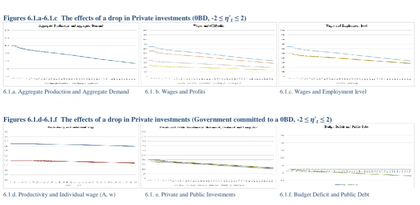
3.6.1 Exogenous drop in Private Investments with a Government committed to 0 Budget Deficit policy ... 59

3.6.2 Who controls the (broad or tight) expectations boundaries? ... 61

3.6.3 Exogenous drop in Private Investments with a moderate Government intervention ... 62

3.6.4 Exogenous drop in Private Investments with a Proactive Government ... 63

3.6.5 Exogenous increase in productivity and real wages under different fiscal policies ... ... 65

3.6.6 Exogenous increase in productivity and real wages with proactive fiscal policies ... ... 66

3.7 Policy implications ... 68

Conclusions ... 69

Bibliography ... 70

- Chapter III - Appendix - The stabilising role of the Government in a Dynamic Distribution Growth Model 71 3.1.A System of Equations ... 71

3.2.A Kaleckian Investment function and firms’ driving force ... 73

3.3.A The Government into the Scene: goals and fiscal policies ... 74

3.4.A BOX 1. Production and utilization function ... 75

3.5.A Eta (𝜼) Analysis: Figures 5.0.a - 5.0.n ... 77

3.6.A Analysis of Initial Equilibrium State and Parameters ... 78

3.7.A Analysis of Key Parameters: ... 79

- Chapter IV- The distributive monetary analysis of a sustainable ecological economy... 81

4.1 Introduction ... 82

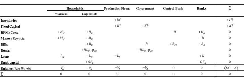
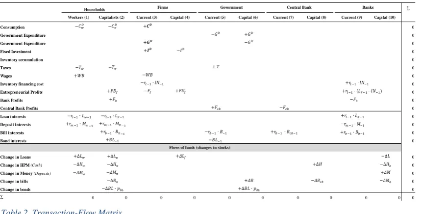
4.2 Balance Sheet and transactions-flow matrix ... 84

4.3 A sketch of the economy ... 86

4.3.1 The endogenous money framework ... 86

4.3.2 The ecological framework of the society ... 87

4.3.3 Firms’ production and investment relations ... 89

4.3.4 Employment, Costs and Wage-Profit determination ... 91

4.3.5 Consumption and households’ relations ... 93

4.3.6 Public Sector relations ... 97

4.3.7 The banking sector relations ... 100

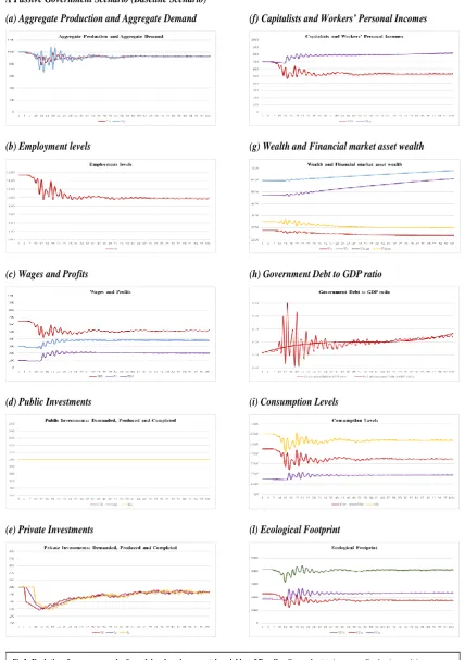
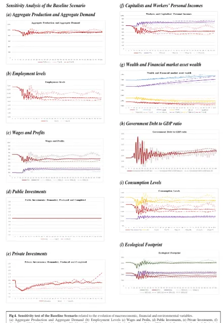
4.4 The effects of a crises on socio economic and ecological distribution ... 101

4.4.1 A passive government scenario ... 102

4.4.2 A 0BD government policy scenario ... 103

4.4.3 A proactive government scenario ... 109

4.5 Policy recommendations and conclusions ... 112

Bibliography ... 115

- Chapter V - Concluding remarks ... 117

- Chapter I -

The State again, an overview

February 14, 2019

The overall goal of this work is to study the effect of a crisis on the distribution and employment

and the space of manoeuvre of the government for supporting and reverting the negative shock

produced by such a crisis. Every chapter of this work and the related models are supported by

both a theoretical background analysis and by numerical dynamic simulations.

Stylized facts show that the income and wealth inequality in all the OECD countries has been

constantly increasing after the 1960s. Piketty has been one of the most important authors that

highlighted the rising inequality issue, mainly in the OECD countries. For example, Piketty (2014)

shows that the income share held by the top percentile in countries such as US, Canada and UK

increased from 8%-10% in the 1960s up to 14%-18% in the current decade. Similar figures are

now provided by the World Inequality Lab1 _{that has updated data for almost every country up to}

2016. At the same time, the wage share for the majority of the OECD countries substantially

decreased. For example, countries such as Italy and Spain experienced a decrease in wage share

from about 73% in the 1970s to about 63% in the current decade (Hein, 2014).

Taking into account such a stylized fact, we will consider a model with two social classes,

workers and capitalists. These social classes differ in terms of their initial endowment, their

consumption behaviour, the different loans repayment conditions required to them by the banks

and in terms of the ways in which they can use their financeable wealth. This is a very important

departure hypothesis from the mainstream point of view models that generally consider a

population made up of “a representative agent” of the whole society.

Considering the inequality levels that the OECD countries are experiencing, we took the

Post-Keynesians school of thought as a very good reference point since it always focused its attention

on the relation between the level of employment, the aggregate demand and the distribution

between social classes. In line with the post-Keynesians tradition, we believe that a theory cannot

be correct unless it starts from realist or realistic hypotheses, although it is recognized that

assumptions are always abstractions and simplifications (Lavoie, 2014).

Therefore, we developed a step by step model with the analysis of an economy based on some

well-known stylized facts. Beyond the social classes distinction, we take into consideration the

temporal lag between production and sales of products by firms and the one between income

received by the social classes and their expenditure. Those two temporal lags are the very key

aspects we focus our attention on in the model presented in Chapter II named “Keynes, Kalecki

and Metzler in a Dynamic Distribution Model”.

In that chapter, we merge the hints of Keynes and Kalecki about the distribution of social

classes and the intervention of the government in supporting the aggregate demand together with

Metzler’s hint about the mismatching process between aggregate demand and aggregate production. Metzler’s mismatching process would finally generate inventories of consumption

goods. More specifically, it is argued that even if Post-Keynesians models focused their attention

on output growth, employment and income distribution relating those issues with a stronger

intervention of the state, they all (even the canonical Kaleckian model) overlooked the adjustment

- or non-adjustment - dynamics from the ultra-short run to the short run period upon which the

short run and long run models are then constructed.

In fact, even if the Kaleckian models completely reject the standard neoclassical production

function (rejecting diminishing returns and rejecting the substitution between capital and labour)

they also very strongly rely on a final equilibrium between aggregate demand and aggregate

production. The canonical Kaleckian short run models are constructed upon the consideration of

the effective labour demand curve defined as “the locus of combinations between real wages and

levels of employment which ensure that all produced goods are sold at the price set by firms”

(Lavoie, 2014). As argued by Lavoie (2014), this construction assures that an increase of real

wage leads to an increase in the employment level. That has been and still is definitely one of the

cornerstones for the Post-Keynesian authors.

We argue that the equilibrium assumption between the aggregate demand and the aggregate

production plays a key role in obtaining the standard Kaleckian conclusions regarding the relation

between effective demand, employment levels and the distribution of surplus product between

the social classes. The main question arising from the previous enquiring exercise about

adjustment dynamics in the Kaleckian framework is that, because of the overlooking on that

adjustment process between aggregate production and aggregate demand, also its conclusions

might be consequentially affected. More precisely the main Post-Keynesian Kaleckian

conclusions to assess are the following: would it still be true that higher real wages lead to a higher

level of employment? Would it still be true that a decrease in the propensity to save will lead to

from falling, whenever there is an increase in productivity there must be some increase in real

wages? And finally, most importantly in terms of policies, would it still be true that in order to

keep employment from falling, even when the economy faces a pari passu increase of real wage

and productivity level, it would be necessary an increase in real autonomous expenditure such as

a strong government one?

In this way, our model analyses under which conditions the standard Kaleckian conclusions

are still valid considering a disequilibrium situation. Two scenarios are simulated: one with fixed

expectations as in Metzler (1941) and another new one based on adaptive expectations and

asymmetric behaviour of the wages-unemployment relation. The model questions the effective

demand labour curve and suggests that an increase in real autonomous expenditures, mainly by

the Government, might be even more essential than what is generally considered in the Kaleckian

literature, to avoid increasing unemployment in an increasing wage world.

The model presented in Chapter III named “The stabilising role of the Government in a

Dynamic Distribution Growth Model” builds upon the model presented in Chapter II and

considers once again the effect of a crises on the relation between aggregated demand,

employment and distribution between social classes adding important characteristics of realism

that were absent in the previous chapter. Here, we consider the gestation period of the investments

and the presence of the government investigating its margin of manoeuvre in such an economy.

The first aspect takes inspiration by Kalecki (1971) himself who considers the three different

Investment stages: investment order or Demand (𝐼𝐷), investment Production (𝐼𝑃) and investment

delivery or Completion (𝐼𝐶). In line with a post-Kaleckian perspective, we consider the expected

profitability and the capacity utilisation as the two main variables as driving forces for the

investment decisions. The second new aspect of this model compared to the one presented in

Chapter II is the explicit presence of the government. In fact, even if chapter II suggested the

Government as the emblematic autonomous figure able to foster expenditure in times of recession,

its actual role in the economy was not analysed. Many post-Keynesian scholars have underlined

how recent decades have been characterised by a strong downgrading of the fiscal policy role as

a stabilisation instrument of macroeconomic policy (Arestis and Sawyer, 2003). In this way, this

chapter analyses exactly the space of manoeuvre of the government and the role of the fiscal

policies into a “functional finance” framework where the government "can and should be called

upon as a key part of the remedy" (Fazzari, 1994) to ensure a high level of economic activity

In the light of such a functional finance framework, the government actions should be inspired

to achieve a more stable and sustainable growth path. More specifically, we here investigate the

possibilities that the Government has to boost and support the economic activity with its two main

tools, public investments spending and a taxation system in two scenarios. The first scenario

simulates an exogenous fall of private investments while the second one relates to an exogenous

increase in labour productivity and real wages. In particular, here we test the canonical Kaleckian

model conclusion according to which even when the economy faces a pari passu increase of real

wages and productivity level it would be necessary an increase in real autonomous expenditures

- such as the one implemented by the government - in order to keep employment from falling.

At the same time, the aim of this chapter is also to explore the role of the Government in

stabilising the economy exactly thanks to the previous tools. In fact, Chapter II underlined the

possibility of an arising unstable path from a mismatching dynamic between aggregate demand

and aggregate production. It was argued that such an unstable path might develop because of

“wrong” oversensitive expectations of firms regarding the production of consumption goods.

Therefore, chapter III focuses exactly on the space of manoeuvre of the government in stabilizing

an unstable economic scenario caused by a crisis.

The model built in Chapter IV named “The distributive monetary analysis of a sustainable

ecological economy” is the natural evolution of the models developed in Chapters II and III. In

such a model all the previous stylized facts are contained, namely the temporal lag between

production and sales of products by firms, the temporal lag between income received by the social

classes and their expenditure, the gestation period of the investments and, finally, the intervention

of the government. The most important difference with respect to the models presented in the

previous chapters is its overall monetary and ecological framework. In fact, for simplification

purposes the previous models were assuming that, in line with a horizontalist approach,

commercial banks were providing funds on demand to firms for financing their investments.

However, the explicit relations among all the sectors of our economy were not fully exposed. In

this chapter Graziani’s endogenous money theory is used and we are developing a Post-Keynesian

Stock Flow Consistent (SFC) model to track all the economic relations, both the real and monetary

ones. At the same time, the use of a SFC model ensures that “there are no black holes - every flow comes from somewhere and goes somewhere” (Godley W. , 1996) through a rigorous accounting

framework, which guarantees a correct and comprehensive integration of all the flows and the

stocks of an economy.

Such as Kalecki, Graziani and the circuitists economists introduce a preliminary distinction

by firms’ decision to activate production and, in order to do so, they take up loans by commercial

banks. In this sense, commercial banks are able to create deposits ex nihilo, granting them loans

and, at the same time, creating deposits. In this way, the starting logical cause of the expansion of

money is exactly the firms’ willingness of contracting a liability to activate production.

In the second step, firms use those loans to pay workers and in this way to obtain the amount

of consumption goods desired through the production process. When such funds are transferred

by firms to households they instantaneously become income paid for the work provided to firms

by workers.

Finally, the last step of the Monetary Circuit is characterized by the households’ spending

decision to use the money balances previously obtained as income. In this step, while households

use their funds to buy consumption goods, firms obtain back those money balances they initially

paid to households for their work.

In this way, the previous Monetary Circuit analysis is not in contrast with the one made by

Kalecki upon the way workers obtain their wages and use all of them to buy consumption goods

while capitalists are able to spend just a proportion of their income.

Finally, together with its social and monetary framework, our economy is also characterized

by an environmental one since we here study the impacts that the economic consumption has in

terms of ecological erosion of natural resources.

In this way, the model of chapter IV questions the expenditure margins of the Government –

in particular after a crisis - and uses the suggestions of the monetary circuit theory to analyse the

space for fiscal policies to reduce unemployment boosting the economic activity, to obtain a more

equitable distribution between social classes in a sustainable ecological way. Our understanding

is that despite many contributions focused on the topics of recovery, distribution and ecological

sustainability, few of them tried to tackle them all in a comprehensive way considering the

rediscovery of the endogenous money phenomena as one of the most important breakthroughs in

the last decades. Here we argue that exactly the endogenous money feature is the essential fil

rouge to better understand and connect the three previous important aspects. It is so when we

analyse the sectors connections and the policies ones devoted to recovery, and also if we consider

how the different incomes and wealth are captured and distributed by the different social classes

and finally when we point out the ways of financing long term ecological path to preserve a

sustainable environment.

Indeed, our overall work in Chapter II, Chapter III and Chapter IV is a step by step construction

of an organic and consistent model. It starts with a more theoretical and simplified approach

suggesting the presence of an autonomous figure such as the government one. Chapter III adds

more real base features through endogenous investments and government presence while Chapter

IV finally concludes considering all the real and monetary links of the sectors into a social and

- Chapter II -

Keynes, Kalecki and Metzler

in a Dynamic Distribution Model

Samuele Bibi

November 21, 2018*

This paper focuses on the dynamics analysis from the ultra-short to the short period from a Post-Keynesian perspective. It is argued that the construction of both the short run and the long run models are based on the critical assumption of an equilibrium between aggregate demand and aggregate supply. Starting from the work by Metzler (1941), the issue of equilibrium and stability is investigated inside a Keynesian-Kaleckian perspective. The suggested model analyses under which conditions the standard Kaleckian conclusions are still valid considering a disequilibrium situation. Two scenarios are simulated: one with fixed expectations as in Metzler (1941) and another based on adaptive expectations and asymmetric behaviour of the wages-unemployment relation. The model questions the effective demand labour curve and suggests that an increase in real autonomous expenditures, mainly by the Government, might be even more essential than what is generally considered in the Kaleckian literature, to avoid increasing unemployment a world with increasing wages.

Key words: Kalecki, Post-Keynesian Economics, Disequilibrium, Adjustment dynamics

JEL classifications: B5, E11, E12, E32

“It is necessary to “think dynamically”. The static system of equations is set not only for its own beauty, but also to enable the economist to train his mind upon special problems when they arise. A new method of approach – indeed, a mental revolution - is needed.”

(Harrod, R.F., 1939: 15)

2.1 Introduction

The Post-Keynesians have always focused on issues such as output growth, employment and

income distribution and, in the last decade, Kaleckian models were developed to show the

* _{This paper has been submitted to the Cambridge Journal of Economics in the date indicated and accepted.}

relevance of the previous issues in justifying a stronger intervention of the state and stronger

public policies. It is argued that while those models reject Say’s law, even the canonical Kaleckian

one overlooked the adjustment - or non-adjustment - dynamics from the ultra-short run to the

short run period upon which the short run and long run models are constructed. Lavoie (1996) is

one of the most audacious attempts to focus on the traverse from one equilibrium position to

another, tackling the adjustment dynamics and considering the effect of hysteresis. However, in

general, all disequilibrium ultra-short-period states are left aside, assuming that “the period under

consideration is long enough for firms to adjust their production to actual demand, and hence that

the economy always operates on the effective labour demand curve” (Lavoie, 2014).

The main question arising from the previous exercise about adjustment dynamics in the

Kaleckian framework is that, because of overlooking that adjustment process, conclusions are

affected consequentially. More precisely, would it still be true that higher real wages lead to a

higher level of employment? Would it still be true that a decrease in the propensity to save will

lead to an increase in output and employment? Would it still be true that in order to keep

employment from falling, whenever there is an increase in productivity there must be some

increase in real wages? And finally, most importantly in terms of policies, would it still be true

that in order to keep employment from falling, even when the economy faces a pari passu increase

of real wage and productivity level, it would be necessary an increase in real autonomous

expenditures such as a strong government one?

This paper proceeds as follows. Section 2 retraces the Post-Keynesians models of short run

and long run focusing on the Kaleckian one. Section 3 suggests a reconsideration of the dynamics

process including some of Metzler’s suggestions in a Keynesian-Kaleckian framework. Section

4 develops a set of preliminary simulations to assess the robustness of the standard Kaleckian

conclusions. Section 5 draws together the conclusions.

2.2 The canonical Short Run and the Long Run Post-Keynesian Kaleckian models

To analyse the relation among the level of employment, the aggregate demand and the distribution

between classes of an economy within a Post-Keynesian framework Kaleckian models are

generally proposed. These are based on the analysis of the effective demand constraint – the

consideration that aggregate supply needs to be equal to aggregate demand.

Kaleckian models reject standard neoclassical production function. They reject diminishing

returns (assuming constant marginal costs -up to full capacity - and therefore constant or

brilliantly the labour peculiarities with respect to capital and the consequent need to reject the

neoclassical production function.

We will focus our attention on retracing the canonical Kaleckian model of short period and

after that on the related adjustment process from the short to the long period as presented “by

textbook” up to this day. We will briefly go back over the previous path as it is presented by

Lavoie (2014) - one of the most important as well as accurate and widely used Post-Keynesian

economics textbooks.

2.2.1 Retracing the canonical Short Run Kaleckian model

The Kaleckian model is generally presented considering a closed economy without any

Government presence where, therefore, the components of the aggregate demand are

consumption and investment. From the consideration of GDP on the expenditure and distribution

side, at the end of each economic period, we can rely on the following identity:

𝑌 = 𝐶𝑜𝑛𝑠𝑢𝑚𝑝𝑡𝑖𝑜𝑛 + 𝐼𝑛𝑣𝑒𝑠𝑡𝑚𝑒𝑛𝑡 = 𝑊𝑎𝑔𝑒𝑠 + 𝑃𝑟𝑜𝑓𝑖𝑡𝑠 (1)

In a Keynesian and Kaleckian view, some of the components of the aggregate demand are

autonomous and some of them are induced. Consumption is made of consumption from wages

𝐶_𝑤 - and consumption from profits - 𝐶_𝜋.

Taking the basic version of the model (and the original assumption by Kalecki), it is assumed

for simplicity that workers consume entirely their wages with a marginal propensity to consume

equal to one (𝑐𝑤 = 1) not being able to save. The aggregate demand is then composed of an

endogenous component related to the wages obtained by workers and an autonomous component

made of consumption out of capitalists and of investment expenditure.

𝐴𝐷 = 𝑤𝐿 + 𝐴 = 𝑤𝐿 + 𝑎𝑝 (2)

being w the nominal wage rate, 𝐿 the amount of employment, 𝑎 the real autonomous expenditure,

𝑝 the price level (and therefore 𝐴 being the nominal autonomous expenditure).

On the supply side, the Kaleckian model does not have a proper production function. It is

replaced by a “utilization function”. Assuming only direct labour use (the labour proportional to

production), the aggregate supply equation would be the following one:

𝐴𝑆 = 𝑝𝑞𝑠_{= 𝑝𝐿𝑦 (3)}

In (3) the quantity obtained in the production process is a direct function of the labour employed

(L) and of the labour productivity (y, here assumed constant). Here production and supply periods

are implicitly considered overlapping, meaning that what is supplied in a certain period is

takes time and a mismatch of the production-supply periods might occur. An implicit

simplification is therefore used making them exactly overlap.

Equating aggregate demand and aggregate supply – (2) and (3) – into (4), we find the effective

demand constraint - equation (5) -, or the effective labour demand curve. That is defined as “the

locus of combinations between the real wage and the level of employment that ensure that

whatever is being produced is sold… such that the goods market is in equilibrium” (Lavoie, 2014).

𝐴𝐷 = 𝐴𝑆 (4)

(𝑤 𝑝⁄ )𝑒𝑓𝑓 = 𝑦 − 𝑎

𝐿 (5)

Equation (5) can be reversed and written as an employment function (6):

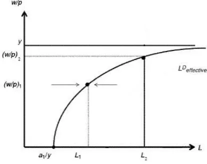
𝐿𝐷_{𝑒𝑓𝑓 =} 𝑎

𝑦 − (𝑤_𝑝) (6)

Obviously, equations (5) and (6) describe the same scenario. As figure 2.1 shows, the Kaleckian

labour demand curve is reflecting an upward sloping labour demand curve - until full capacity

utilization.

Figure 2.1. The Kaleckian post-Keynesian model of employment. Source: Adapted from Lavoie, 2014, p. 293

Once the Kaleckian model structure has been presented, the adjustment process of production to

demand is explained as follows:

As long as firms react to a situation of excess supply (demand) on the goods market by reducing (increasing) production, rather than changing the mark-up and hence prices, the economy will move horizontally towards the locus of equilibria, that is, towards the effective labour demand curve. In other words, the model exhibits stability under these conditions. Henceforth we will presume when doing comparative analysis, that the period under consideration is long enough for firms to adjust their production to actual demand, and hence that the economy always operates on the effective labour demand curve (emphasis added).

As a consequence of the previous argument, some fundamental conclusions have been proposed

(Lavoie, 2014, p.295-297):

1) “Higher real wages will generate more employment”. This could be so for different

reasons such as a higher nominal wage claim by workers not followed by the same

increase in prices. In a different way, the increase of real wages could be due to a

decreasing mark-up applied by the firms (due, for example, to higher competition in the

market) not followed by the same speed in the reduction of prices. Whatever the trigger

of the real wage increase, that would lead to a higher level of employment thanks to the

employment multiplier effect, as explained in Lavoie (2014).

2) An increase in the propensity to save out of profit will lead to a reduction in output and

employment.

3) In order to keep employment from falling, whenever there is an increase in productivity

there must be some increase in real wages.

4) In order to keep employment from falling and avoid technological unemployment, even

when the economy faces a pari passu increase of real wage and productivity level, there

should be an increase in real autonomous expenditure such as a strong government

expenditure.

“The canonical Kaleckian model of growth and distribution” is then presented by considering the dynamic version of the principle of effective demand that is the “equilibrium locus on the goods market, by equating aggregate supply with aggregate demand” (Lavoie, 2014). Exactly equating

aggregate supply with aggregate demand will imply investments are equal to savings.

𝐼 = 𝑆 (7)

The canonical Kaleckian long run model is then based on the dynamic version of equation (7):

𝑔𝑖 _{= 𝑔}𝑠

(8)

where 𝑔𝑖 is the rate of growth of investment and 𝑔𝑠 is the rate of growth of savings.

It is therefore evident how both the canonical short run as well as the long run Kaleckian

models are constructed on the equalization between aggregate demand and aggregate supply. That,

in turn, is based on an adjustment mechanism that leads the economy exactly on its effective

demand curve. In short, everything must ultimately converge.

Although this convergence process could possibly and eventually take place, to assume that is

far from obvious, straightforward and innocuous. In this sense, if even Kaleckians have often

the stability and adjustment analysis by studying under which circumstances some of the usual

corollaries may be nuanced.

2.2.2 Questioning the canonical Kaleckian short run and long run models

The last part of Lavoie (2014) sentence quoted in Section 2.1 shows how, in general,

Post-Keynesian economists leave aside a computational analysis of the adjustment process in the

ultra-short period. Lavoie (1996) is one of the most audacious attempt to focus on the traverse from

one equilibrium position to another, tackling the adjustment dynamics and considering the effect

of hysteresis. However, in general, the assumption of the economy being already in the short

period in the Kaleckian model explanation is made. Lavoie (2014) suggests that “ideally, a formal

model would take into account changes in inventories” and the aim of Section 3 will be exactly

to build a computational model analysing the adjustment (or non-adjustment) process in a

Kaleckian framework by considering the time lags in more detail.

Our analysis starts with the equilibrium condition between the aggregate actual demand and

the aggregate supply (4). Now, simply by substitution, from (4), equation (6) can be easily derived

through the following steps:

If and When AD = AS (4)

𝑤𝐿 + 𝑎𝑝 = 𝑝𝐿𝑦 (9)

𝑤

𝑝𝐿 + 𝑎 = 𝐿𝑦 (10)

𝐿 (𝑦 −𝑤

𝑝) = 𝑎 (11)

Then 𝐿𝑒𝑓𝑓

𝐷 ₌ 𝑎

𝑦 −𝑤_𝑝 (6)

Following the previous steps, it could be argued that iff aggregate demand is equal to

aggregate supply (4) we would obtain the effective labour demand curve as described in figure 1.

In fact, when (4) is not assured, the economy could be oscillating with stability around it (in a sort

of mismatching situation between aggregate supply and aggregate demand), fluctuating with an

implosive or explosive behaviour, or even without an increasing curve at all. The potential

indeterminability of such an effective labour demand curve could undermine not only the

example, not having an effective demand curve with the shape of figure 1 could mean

undermining the conclusion 1 previously cited according to which higher real wages will generate

more employment.

Although we consider the presentation of the canonical Kaleckian model extremely important

in the Post-Keynesian literature, further helpful insights could be gained by using an algorithmic

procedure. Our first research question concerns the main canonical Kaleckian model conclusions

explained excellently in Lavoie, 2014, p. 295-298. More specifically such research questions are

linked to the following issues:

1) Can we be sure and assume that (already in the short run and then more in general) the

economy reaches and stays on the effective labour demand curve?

2) Would it still be true that higher real wages lead to a higher employment? This point is

linked to the paradox of costs.

3) Would it still be true that an increase in the propensity to save will lead to a reduction in

output and employment? This point directly refers to the paradox of thrift.

4) Would it still be true that in order to keep employment from falling, whenever there is an

increase in productivity, there should be some increase in real wages?

5) Would it still be true that in order to keep employment from falling, even when the

economy faces a pari passu increase of real wages and productivity level, it would be

necessary an increase in real autonomous expenditures such as one implemented by the

government?

2.3 The ultra-short run reconsidered: an alternative dynamic analysis

To tackle the fulfilment of the effective demand constraint, we have to consider what this implies:

the equality between aggregate demand and aggregate supply. The effective demand is generally

defined as “the locus of combinations between real wages and levels of employment which ensure

that whatever is being produced is sold at the price set by firms” (Lavoie 2014, p. 282).

As discussed above, to suppose that we already are on the effective demand curve or that “the period under consideration is long enough for firms to adjust their production to actual demand”

is like considering we have hit directly upon the effective demand curve without truly computing

a real reaction (and not necessarily adjustment) mechanism. Once we believe we are on the

effective demand labour curve, moving along that is like considering we got stuck in a

not allowing the possibility for the economic system to constantly be off that path or to deviate

once we are on it.

The keystone of inventories analysis is the work done by Metzler (1941). Metzler himself

considers two types of time relations: a “Robertson or Receipt-Expenditure lag” and a “Lundberg

or Sales–Output lag”. The former refers to “the lag in the expenditure of income behind its receipt”

(Metzler, 1941). The latter “Lundberg S-O” lag refers instead to the existing lag between the

change in revenue from sales and the output of consumer goods. “In other words, businessmen

were assumed to base their production in period t upon sales in period t-1” (Metzler, 1941). This

lag is the one that generally produces an impact on inventories. Although Metzler himself stresses

the relevance of both lags, he finally prefers to focus only on the Lundberg S-O lag.

2.3.1 The core assumptions of the model and national identities

In contrast to Metzler, we will try to merge the two types of lags, since we consider both lags are

more representative of the current real world situation.

Before considering the reaction (and not necessarily adjustment) mechanisms implicit in the

described lags, we will try here to disentangle the forces that lie behind the aggregate production

by firms and the ones tied to aggregate demand. This would not necessarily imply that everything

produced by firms is actually sold, thus giving rise to inventories through time.

Most precisely, and in the spirit of Metzler analysis too, we claim that at least three main forces

might lead aggregate production to diverge from aggregate demand: the multiplier mechanism,

the accelerator mechanism and the role of expectations.

Beyond the simulation itself related to the suggestions within the framework proposed by

Metzler, the features merged in a Kalecki-Metzler framework are the following ones:

a. the presence of different social classes, more specifically workers and firms;

b. the fact that collective bargaining (instead of the market) forces are the ones behind the

wage-profit distribution between workers and firms;

c. different marginal propensity of consumption between the two predominant social

classes–workers and capitalists.

d. Finally, in accordance with both Kalecki and Metzler, we will suppose that firms react to

the demand side stimulus through quantity variation and not through the price one. This

adequate inventories so that any discrepancy between output and consumer demand may

be met by inventory fluctuations rather than price changes” (Metzler, 1941).

That is why, in accepting this hypothesis made both by Kalecki and Metzler, we will assume that

prices are constant. Constant prices means that a definite price level is the one at which firms are

ready to sell their product in a certain period.

We will now propose the main structural and behavioural equations that represent the main

relations and reaction mechanisms in this framework both in real and in nominal terms. Since the

price level is here considered constant and we can assume p=1, the price variable will not appear

in the following equations.

𝑌𝑡𝑃= 𝐶𝑡𝑃+ 𝐼𝑡𝑃 (12)

The total production in a given period is mainly composed by the production of Consumption

goods - 𝐶𝑡𝑃- and production of Investment goods - 𝐼𝑡𝑃 – in a certain period. The production

process is carried out by the firms that hire and pay the workers. Here the superscripts P stand for

the produced side of the previous aggregate values.

𝑌_𝑡𝑁𝐼 _{= 𝑊}

𝑡+ 𝛱𝑡 (13)

The National Income of a country in a period - 𝑌𝑡𝑁𝐼 - is shared by the aggregate level of wages -

𝑊_𝑡 - and the aggregate level of profits - 𝛱𝑡. 𝑌_𝑡𝐷_{= 𝐶}

𝑡𝐷+ 𝐼𝑡𝐷 (14)

The total amount of product demanded in a period - 𝑌_𝑡𝐷- is composed by the aggregate demand

for Consumption goods - 𝐶𝑡𝐷- and by the aggregate demand for Investment goods - 𝐼𝑡𝐷. Here the

superscripts D stand for the demanded side of the previous aggregate values. For the moment, we

will consider the investment component as fixed.

𝑌_𝑡𝑃_{= 𝑌}

𝑡𝑁𝐼 (15)

The total income produced in a certain period - 𝑌𝑡𝑃 - is paid out to the social classes - 𝑌𝑡𝑁𝐼

considered aggregated into workers and capitalists or firms. Here, it is important to underline that

we are no longer supposing that the Production obtained in one year is totally sold absorbed by

the aggregate Demand. In this way, firms production - 𝑌_𝑡𝑃- might well be different from goods

demanded in a period - 𝑌𝑡𝐷 - thus possibly giving rise to the inventories issue.

2.3.2 Consumption and Production relations

𝐶_𝑡𝐷_{= 𝐶}

𝑡 𝑤𝐷 + 𝐶𝑡 𝜋𝐷 (16)

The aggregate Demand of Consumption goods - 𝐶_𝑡𝐷 - is made up of two parts: the Demand of

Consumption goods by workers- 𝐶𝑡 𝑤𝐷 - and the Demand of Consumption goods by capitalists -

𝐶_{𝑡 𝜋}𝐷 _{. In line with Hansen and Samuelson, we will firstly assume that the Demand of Consumption}

goods for a certain period is related to the receipts obtained in the previous one. We will assume

that for both consumers and for capitalists.

𝐶_{𝑡 𝜋}𝐷 _{= 𝐶}

0𝜋+ 𝑐𝜋 𝛱𝑡−1 (17)

Hence, the Demand of Consumption goods by capitalists includes an exogenous component - 𝐶0𝜋

- and a part - 𝑐𝜋 𝛱𝑡−1 - linked to the profits obtained in the previous period by the capitalists

through their specific marginal propensity (𝑐𝜋).

𝐶_{𝑡 𝑤}𝐷 _{= 𝐶}

0𝑤+ 𝑐𝑤 𝑊𝑡−1 (18)

In turn, the Demand of Consumption goods by workers is also partly composed by an exogenous

component - 𝐶0𝑤 - and a part - 𝑐𝑤 𝑊𝑡−1 - linked to the wages obtained by the workers in the

previous period through their specific marginal propensity (𝑐𝑤).

𝐶_𝑡 𝑃_{= 𝐸}

𝑡−1(𝐶𝑡 𝐷) + 𝑠𝑡∗ (19)

Equation (19) represents the basic Lundberg S-O hypothesis according to which businessmen

base their production in period t upon sales in period t-1. This is done through the role of

expectations (𝐸_𝑡−1) upon the demand for consumption goods to be produced for the following

period (𝐶_𝑡 𝐷), the functional form of which will be underlined in equation (20). In addition, it is

then assumed that, more than producing for what they expect to sell in the following period, firms

also produce a certain desired level of inventories, 𝑠∗(𝑡). This hypothesis is in line with many

post-Keynesians authors who have tackled the issue of inventories. Godley and Lavoie (2007a),

for example, argue that firms do want to produce a target level of inventories because of

uncertainty.

The functional form of the desired inventories (24) plays an important role in the determination

of production.

𝐸_𝑡−1(𝐶𝑡 𝐷) = 𝐶𝑡−1 𝐷 + 𝜂(𝐶𝑡−1𝐷 − 𝐶𝑡−2𝐷 ) (20)

𝜂𝑡 =

𝐶_𝑡𝐷_{− 𝐶} 𝑡−1𝐷 𝐶_𝑡−1𝐷 _{− 𝐶}

𝑡−2 𝐷

(21)

𝐸𝑡−1(𝐶𝑡 𝐷) = 𝐶𝑡−1 𝐷 + 𝜂′(𝐶𝑡−1𝐷 − 𝐶𝑡−2𝐷 ) (22)

𝜂′_𝑡=𝐶𝑡−1

𝐷 _{− 𝐶}

𝑡−2 𝐷 𝐶_𝑡−2𝐷 _{− 𝐶}

𝑡−3 𝐷

The specification of the expectation equation (20) is derived from the latest model proposed

by Metzler himself. In that model, instead of considering the expected sales of the next period to

be simply equal to the consumption goods demanded in the previous one, another component is

added. As he says: “expectations of future sales may depend not only upon the past level of sales, but also upon the direction of change of such sales” (Metzler, 1941). We should therefore consider another component in the expectation, a “trend cycle projection” according to which firms will

take into account the trend of the last two – for instance - production periods, perceiving that the

same demand trend will be maintained or instead – guessing that the end phase of a cycle is

arriving – reversed. Following Metzler, we called this coefficient of expectations “𝜂”. In Metzler

(1941), it represents “the ratio between the expected change of sales between periods t and t-1

and the observed change of sale between period t-1 and t-2” (Metzler, 1941). It is represented by

equation (23). Following the Metzler explanation, we will consider the value of 𝜂 lying between

-1 and 1.

Later, we will slightly change the composition of 𝜂, suggesting that it embodies the same ratio

but lagged one period back, that is to say “the ratio between the observed change of sales between

periods t-1 and t-2 and the observed change of sale between period t-2 and t-3”. We will call “η′”

(equation (23)) that modified version of η. Taking η′ into account it will produce equation (22)

that will then replace equation (20). In this behavioural equation, the production of demanded

goods is therefore partly related to the demand of the previous year and partly assumed to be a

linear function of the rate of change of the demanded goods in the last two (or further on, three)

periods - this is related to the Hansen-Samuelson acceleration principle.

𝑠_𝑡∗_{= 𝛼 𝐸}

𝑡−1(𝐶𝑡 𝐷) − 𝑄𝑡−1 (24)

Equation (24) represents the desired level of inventories that firms intend to produce or the

desired change in inventories. Instead of considering their attempt in maintaining a certain level

of constant inventories, it is assumed that the latter is related to the expected level of sales. More

specifically, as to inventories, we suppose that entrepreneurs try to maintain those at a constant

proportion of the expected sales of the next year’s demand. Following Metzler’s suggestion, we

will call 𝛼 that proportion. The idea of a targeted or desired proportion of inventories is widely

accepted in the Kaleckian literature that tackles the inventories issue and it could be associated

with the Godley-Lavoie target inventories to sales ratio, 𝜎𝑇 (Godley & Lavoie, 2007a).

𝑄𝑡 = 𝑠𝑡+ 𝑄𝑡−1= 𝐶𝑡 𝑃− 𝐶𝑡 𝐷+ 𝑄𝑡−1 (25)

Finally, the total amount of inventories stocked at the end of a certain period - 𝑄𝑡 - is simply

existing in the previous one 𝑄𝑡−1. In turn, the former is the discrepancy between the Production

of Consumption goods and the Demand of Consumption goods, 𝐶𝑡 𝑃− 𝐶𝑡 𝐷. It is important to

underline that the actual inventories level - 𝑠𝑡 - in a certain period might well be different from

the desired one - 𝑠𝑡∗.

The following equations are based upon Blanchard et al. (2010) but they are different in many

ways, the most important of which is that the following ones are expressed in a dynamical sense

explicitly considering the timing issue. The other relevant difference refers to the exogeneity or

endogeneity of some variables. Thirdly, almost all of the following equations do explicitly take

into consideration both the real and the monetary aspects. This is done in line with the

Post-Keynesian literature that considers monetary influences having a role in determining the level of

aggregate demand and through that of the employment and economic activity. When we deal with

the monetary issue, it will appear how that is true not only in the “short run” as the mainstream

literature claims.

𝐶_𝑡 𝑃_{= 𝐴}

𝑡𝑁𝑡 𝐶 (26)

The total production in a certain period is given by the total number of workers employed in

the production process 𝑁𝑡 𝐶 multiplied by their productivity 𝐴𝑡.The first really important

distinction with respect to the exogenous variable considered by Blanchard et al (2010) is the one

regarding productivity (𝐴_𝑡). In fact, in that model, the productivity is considered exogenously

given, while we claim that is not the case. We will focus on the productivity aspect later on in

equations (33).

𝑁_𝑡 𝐶 ₌𝐶𝑡 𝑃

𝐴_𝑡 (27)

Equation (26) can obviously be converted into (27) that shows how employment in an

economy is positively related to its total production.

2.3.3 Wages and Profits relations

In this subsection, the relations at the base of wages and profits determination will be presented.

The following equation is also based on Blanchard et al. (2010).

However, there are important differences between (29) and the one proposed by Blanchard

such as the assumption of constant prices (for the reasons given in subsection 3.1) and the fact

that it is the individual (not the collective) nominal wage to be function of the expected prices,

unemployment and z (workers’ protection laws). For now, anyway, we are supposing fixed prices

𝑤𝑡 = 𝑤𝑡−1+ 𝛾𝑧

𝑧_𝑡− 𝑧_𝑡−1

𝑧𝑡−1 𝑤𝑡−1− 𝛾𝑢(𝑢𝑡−1− 𝑢𝑡−2)𝑤𝑡−1 (28)

𝑊𝑡 = 𝑤𝑡 𝑁𝑡 𝑇 (29)

Equation (28) assumes individual real wage claimed by workers in a certain period based on the

previous one. Workers will then adjust that taking into account the variables previously

considered. The parameters 𝛾𝑧 and 𝛾𝑢 reflect the sensitivity of the wage claim with respect to the

protection of the workers.

It is assumed that the demanded wage is negatively related to the unemployment rate of a certain

period and context, 𝑢𝑡

𝑁_𝑡 𝑇 _{= 𝑁}

𝑡 𝐶+ 𝑁𝑡 𝐼 (30)

Equation (30) represents the total number of workers employed in a certain period in the economy.

This is the sum of the workers employed to produce consumption goods, 𝑁_𝑡 𝐶, and producing

Investment goods, 𝑁𝑡 𝐼.

𝑁𝑡 𝐼 = 𝐼_𝑡 𝑃

𝐴𝑡 (31)

As well as equation (27), equation (31) represents the number of workers employed in producing

the private Investments goods.

𝑢_𝑡=𝑈𝑡 𝐿 =

𝐿 − 𝑁_𝑡

𝐿 = 1 −

𝑁_𝑡 𝑇 𝐿 = 1 −

𝑌_𝑡 𝑃

𝐴𝑡 𝐿 (32)

The rate of unemployment of a certain period, 𝑢𝑡, is simply given by the ratio between the total

amount of unemployed people, 𝑈𝑡, and the total labour force, L, that we start considering as fixed.

It is important to point out that labour productivity (𝐴𝑡) should not be considered an exogenous

value determined outside the economic system. In truth, many studies suggest that labour

productivity is related to different features. For example, Schor (1987) found that work effort is

influenced by the wage rates level, by the rate of unemployment or the average duration of

unemployment, and by the presence of social security benefits. We could also recall the Webb

effect that relates real wages and labour productivity. In this line, Marquetti (2004)

econometrically shows the existence of a unidirectionality relation from the former to the latter.

Also social influences such as work satisfaction should be taken into account. Akerlof (1982)

suggests that higher wages or higher wages compared to other groups of workers stimulate

satisfaction and, through that, a better work environment and higher productivity. Recent works

established and documented a positive relation between wage claims and labour productivity the

former being the determinant of the latter.

By the same token, Kleinknecht et al. (2016) argue that the positive incidence of wage protection

upon labour productivity works in different ways.

Invoking the Webb effect supported by Marquetti (2004), labour productivity is then considered

as a positive function of real wage, as described by equation (33):

𝐴𝑡 = 𝐴𝑡−1+ 𝛾𝜔(

𝜔_𝑡− 𝜔_𝑡−1

𝜔_𝑡−1 ) 𝐴𝑡−1, (33)

Finally, it is important to analyse the concept of profits more fully to underline a crucial aspect:

the difference between the profit in its accountability terms and in the cash flow one. Appendix

3.3 sets out details on the inventories analysis and on its consideration in the accountability profit.

According to the accountability profits aspect, the inventories from a certain period are included

in the profits obtained by capitalists. This is so because the inventories will be sold in future

periods and since we are considering a model where prices are fixed, the evaluation of the

inventories problem should not arise: their value would not change. In this way the production

obtained at the end of each period will be completely shared among the social classes – wages to

workers and profits to capitalists. However, in accounting terms, the latter now includes the

inventories produced. This is the way profits are considered in equation (34).

𝛱𝑡 = 𝑌𝑡𝑃− 𝑊𝑡 (34)

In terms of the cash flow profit, we can clearly separate the effective amount of profits obtained

and spendable by capitalists from the residual inventories at the end of the process. According to

this frame and since the unsold production will give rise to the inventories, the production

obtained at the end of each period will not be completely shared among the social classes. The

national income actually distributed will be therefore the net production value of the inventories

(the term between parenthesis in equation (35)), producing the following equation.

𝑌_𝑡𝑁𝐼_{= 𝑌}

𝑡𝑃− (𝑌𝑡𝑃− 𝑌𝑡𝐷) (35)

that obviously reduces to the following (36):

𝑌_𝑡𝑁𝐼_{= 𝑌}

𝑡𝐷 (36)

Putting equation (36) into (13), we finally obtain the profits received by capitalists in terms of

cash flow (37), П_𝑐𝑓, underling the actual amount of resources they dispose of.

2.4 Preliminary Simulations

From now on, because of the issues proposed in section 3 and discussed in details in appendix

3.3, we will consider the Profits in the Cash Flow Profits meaning as defined in equation (37)2.

In this model, the investments are not explained but they are simply considered as exogenously

given. Furthermore, it is assumed that there is no Government presence in the economy and that,

in line with a horizontalist approach, commercial banks provide funds on demand to firms for

financing their investments. Prices are considered constant. We will consider a modified version

of Metzler expectations (1941).

In fact, Metzler (1941) offered some strong implicit simplifications as to expectations

regarding the constancy of the respective parameter and the boundaries the parameter itself

assumed. In particular, despite producers’ expectations being taken into account, 𝜂 was finally

considered as a constant value along with the traverse and dynamics, in this way attributing the

same weight to the expectation of the demand in the different periods. In light of that, a slightly

different coefficient of expectation - 𝜂′ - will be considered, the value of which should be left free

to vary between reasonable boundaries levels. The value of 𝜂′ still embodies the same ratio of 𝜂

but now lagged one period back, to allow the expectation parameter to vary. In this way, producers

will still have expectations according to the recent past (we considered the past three periods)

having 𝜂′ the form considered in (23). We would allow 𝜂′ to vary freely within acceptable

boundaries (𝜂′𝐿 𝑎𝑛𝑑 𝜂′𝑈) described by equations (23𝐿) - (23𝑈).

The second change we allow to our expectations with respect to Metzler (1941) regards the

boundaries values the related parameter might take. In fact, the analysis of figures (4.0.a-4.0.n)

allows us to appreciate that considering only the values proposed by Metzler (-1:1) would

implicitly constrain our analysis avoiding those values that exactly describe booms and busts (for

values of 𝜂 higher than 1, figures 4.0.c and 4.0.f) and those ones describing strong reversing

behaviours in the economic cycle (for values of 𝜂 lower than -1, figures 4.0.i and 4.0).

In this sense, our model allows us to include a broader spectrum of values for the expectations

by tackling the previous two aspects. We will then consider our 𝜂′ free to vary between a broader

range (-1,5 and 1,5), where not differently established.

2 _{It can be noted that in case we considered the accounting profit (34) as a main driver of the firms, an increasing level of inventories}

Eta (𝜼) Analysis: Figures 4.0.a - 4.0.n

Figure 4.0.a: Soft increase Figure 4.0.b: Straight increase Figure 4.0.c: Strong increase 𝐶𝑡−2 𝐷 − 𝐶𝑡−3 𝐷 > 0 𝐶𝑡−2 𝐷 − 𝐶𝑡−3 𝐷 > 0 𝐶𝑡−2 𝐷 − 𝐶𝑡−3 𝐷 > 0

𝐶𝑡−1 𝐷 − 𝐶𝑡−2 𝐷 > 0 𝐶𝑡−1 𝐷 − 𝐶𝑡−2 𝐷 > 0 𝐶𝑡−1 𝐷 − 𝐶𝑡−2 𝐷 > 0 𝐶𝑡−1 𝐷 − 𝐶𝑡−2 𝐷 < 𝐶𝑡−2 𝐷 − 𝐶𝑡−3 𝐷 𝐶𝑡−1 𝐷 − 𝐶𝑡−2 𝐷 = 𝐶𝑡−2 𝐷 − 𝐶𝑡−3 𝐷 𝐶𝑡−1 𝐷 − 𝐶𝑡−2 𝐷 > 𝐶𝑡−2 𝐷 − 𝐶𝑡−3 𝐷

Figure 4.0.d: Soft decrease Figure 4.0.e: Straight decrease Figure 4.0.f: Strong decrease 𝐶𝑡−2 𝐷 − 𝐶𝑡−3 𝐷 < 0 𝐶𝑡−2 𝐷 − 𝐶𝑡−3 𝐷 < 0 𝐶𝑡−2 𝐷 − 𝐶𝑡−3 𝐷 < 0

𝐶𝑡−1 𝐷 − 𝐶𝑡−2 𝐷 < 0 𝐶𝑡−1 𝐷 − 𝐶𝑡−2 𝐷 < 0 𝐶𝑡−1 𝐷 − 𝐶𝑡−2 𝐷 < 0 𝐶𝑡−1 𝐷 − 𝐶𝑡−2 𝐷 > 𝐶𝑡−2 𝐷 − 𝐶𝑡−3 𝐷 𝐶𝑡−1 𝐷 − 𝐶𝑡−2 𝐷 = 𝐶𝑡−2 𝐷 − 𝐶𝑡−3 𝐷 𝐶𝑡−1 𝐷 − 𝐶𝑡−2 𝐷 < 𝐶𝑡−2 𝐷 − 𝐶𝑡−3 𝐷

Figure 4.0.g: Soft upward switch Figure 4.0.h: Prop. upward switch Figure 4.0.i: Strong upward switch 𝐶𝑡−2 𝐷 − 𝐶𝑡−3 𝐷 < 0 𝐶𝑡−2 𝐷 − 𝐶𝑡−3 𝐷 < 0 𝐶𝑡−2 𝐷 − 𝐶𝑡−3 𝐷 < 0

𝐶𝑡−1 𝐷 − 𝐶𝑡−2 𝐷 > 0 𝐶𝑡−1 𝐷 − 𝐶𝑡−2 𝐷 > 0 𝐶𝑡−1 𝐷 − 𝐶𝑡−2 𝐷 > 0

𝐶𝑡−1 𝐷 − 𝐶𝑡−2 𝐷 < |𝐶𝑡−2 𝐷 − 𝐶𝑡−3 𝐷 | 𝐶𝑡−1 𝐷 − 𝐶𝑡−2 𝐷 = |𝐶𝑡−2 𝐷 − 𝐶𝑡−3 𝐷 | 𝐶𝑡−1 𝐷 − 𝐶𝑡−2 𝐷 > |𝐶𝑡−2 𝐷 − 𝐶𝑡−3 𝐷 |

Figure 4.0.l: Soft downward switch Figure 4.0.m: Prop downward switch Figure 4.0.n: Strong downward switch 𝐶𝑡−2 𝐷 − 𝐶𝑡−3 𝐷 > 0 𝐶𝑡−2 𝐷 − 𝐶𝑡−3 𝐷 0 𝐶𝑡−2 𝐷 − 𝐶𝑡−3 𝐷 > 0

𝐶𝑡−1 𝐷 − 𝐶𝑡−2 𝐷 < 0 𝐶𝑡−1 𝐷 − 𝐶𝑡−2 𝐷 < 0 𝐶𝑡−1 𝐷 − 𝐶𝑡−2 𝐷 < 0

|𝐶𝑡−1 𝐷 − 𝐶𝑡−2 𝐷 | < 𝐶𝑡−2 𝐷 − 𝐶𝑡−3 𝐷 |𝐶𝑡−1 𝐷 − 𝐶𝑡−2 𝐷 | = 𝐶𝑡−2 𝐷 − 𝐶𝑡−3 𝐷 |𝐶𝑡−1 𝐷 − 𝐶𝑡−2 𝐷 | > 𝐶𝑡−2 𝐷 − 𝐶𝑡−3 𝐷

Cd(t-3) Cd(t-2) Cd(t-1)

0 < 𝜂< 1

soft increase

Cd(t-3) Cd(t-2) Cd(t-1)

𝜂= 1

straight increase

Cd(t-3) Cd(t-2) Cd(t-1)

𝜂> 1 Strong increase

Cd(t-3) Cd(t-2) Cd(t-1)

0 < 𝜂< 1

soft decrease

Cd(t-3) Cd(t-2) Cd(t-1)

𝜂= 1

straight decrease

Cd(t-3) Cd(t-2) Cd(t-1)

𝜂> 1 Strong decrease

Cd(t-3) Cd(t-2) Cd(t-1)

-1 < η < 0

soft upward switch

Cd(t-3) Cd(t-2) Cd(t-1)

η = - 1

prop. upward switch

Cd(t-3) Cd(t-2) Cd(t-1) η < - 1 Strong upward

switch

Cd(t-3) Cd(t-2) Cd(t-1)

-1 < η < 0

soft downward switch

Cd(t-3) Cd(t-2) Cd(t-1)

η = - 1

prop. downward switch

Cd(t-3) Cd(t-2) Cd(t-1) η < -1 Strong downward

𝐸𝑡−1(𝐶𝑡 𝐷) = 𝐶𝑡−1 𝐷 + 𝜂′(𝐶𝑡−1𝐷 − 𝐶𝑡−2𝐷 ) ₍₂₂₎

𝜂′𝑡=𝐶𝑡−1 𝐷 _{− 𝐶}

𝑡−2 𝐷 𝐶𝑡−2𝐷 − 𝐶𝑡−3 𝐷

(23)

𝜂′𝑡= 𝜂′𝐿 𝑖𝑓 𝜂′𝑡> 𝜂′𝐿

(23L)

𝜂′𝑡= 0 𝑖𝑓 𝐶𝑡−2𝐷 _{= 𝐶}

𝑡−3 𝐷 ₍₂₃₀₎

𝜂′𝑡= 𝜂′𝑈 𝑖𝑓 𝜂′𝑡< 𝜂′𝑈 (23U)

2.4.1 Exogenous increase of the Private Investments

A scenario in which the investments exogenously increase is set out. In this case, after the shock

has been introduced, the aggregate demand and production, after a brief and moderate

mismatching between them, tend to come back to an equal (and stable) level again. In fact, such

a positive shock in one component of the aggregate demand (𝐶𝑡 𝐷) pushes up the expectations of

firms, thus increasing their production (𝐶_𝑡 𝑃) through (19). However, since the push in the

component of 𝐶𝑡 𝐷 is just an una tantum increase, the multiplier effect loses its strength and allows

𝐶_𝑡 𝐷 _{to finally stabilize at a higher level. So, the reduced 𝐶}

𝑡 𝐷 increases lead to an oscillation

reduction of the expectation and of 𝐶𝑡 𝑃 the value of which starts to implode until it stabilizes itself

adjusting to the new 𝐶𝑡 𝐷 level.

4.1.a. Aggregate Production and Aggregate Demand 4.1.b. Wages and Profits 4.1.c. Wages and Employment level

Figures 4.1.a-4.1.c The effects of an increase of the Private Investments

In the same way, Profits, Wages and Employment levels tend to stabilize again at higher levels

compared to the initial ones after a brief increase in the first periods. Considering the wage-profits

differential level, it is shown that an exogenous increase of investment leads to a faster increase

2.4.2 The effect of a higher workers’ claims and wages

According to the Post-Keynesian literature, an exogenous increase in real wages (for example due

to higher wage claims by the workers) will increase the level of activity and employment. This is

linked to the famous paradox of costs, mentioned in section 2.2. It is generally claimed that such

a conclusion is still valid when we consider the presence of the Webb effect and also that “the

positive relationship between real wages and the level of employment will persist as long as the

reaction parameter (of productivity with respect to wages - our 𝛾_𝜔 -) is smaller than unity” (Lavoie,

2014).The results here presented are actually not completely in line with that scenario and the

paradox of costs now happens in some constellation of parameters and not in others.

In fact, despite a 𝛾𝜔 lower than 1 (𝛾𝜔 = 0.5), the employment level slightly decreases as a

consequence of an increase of wages level caused by a higher EPL (see figure 4.2.c). Here, a first

and “una tantum” rise in z level, the residual variable summarizing the workers’ protection, causes

increasing wages level claimed by workers. Such an increase has, in turn, two effects: on one side,

it increases workers’ productivity (through the Webb effect we reached with (33)) and as a

consequence, it makes firms hire fewer employees to produce the same amount of consumption

goods. The wage increase also boosts workers’ consumption. If we consider the higher share of

wages as a part of national income and the higher marginal propensity of consumption by workers

with respect to capitalists, all that makes the total demand for consumption goods rise together

with production allowing a partial employment recovery that nevertheless remains lower than the

pre-shock level (figure 4.2.c).

4.2.a. Aggregate Production and Aggregate Demand 4.2.b. Wages and Profits 4.2.c. Wages and Employment level Figures 4.2.a-4.2.c The effects of an increase of EPL (from 80 points in period t=3 to 120 points in t=4) with 𝜸𝝎= 𝟎. 𝟓𝟎 and 𝜼𝒕= 𝟏. 𝟓𝟎

However, once a proper analysis of the interaction of the inventories and the mismatching

between the demand and the production is considered, the causal mechanisms are not as

straightforward as presented. A deeper analysis of the causal relations is presented in appendix

figure 4.2.0. The conclusions of the figure presented generally do vary with respect to several

factors such as the sensitivity of wages to the variation of EPL or workers’ protections (𝛾_𝑧), the

sensitivity of wages to the variation of the unemployment level (𝛾𝑢), the sensitivity of workers’

productivity to variations in wages (𝛾𝜔) and the expectations of firms (𝜂′𝑡). For example, with a

wages and economic activity suggesting that in such a case the paradox of costs still holds (not

reported). The complexity involved in the model allows us to appreciate how the final impact of

employment level depends on the constellation values of the parameters previously mentioned.

The previous scenario presented in figures 4.2.a-c takes into consideration the case in which

there is an “una tantum” increase of the EPL. We could do the same exercise with a “continuous”

increase in z, as if the EPL was going to increase constantly over time due to higher workers’

claims. The result would not be different: in any case, we would obtain the same decreased level

of employment (figures 4.2 d-f, in Appendix) even in cases of a present low Webb effect (𝛾_𝜔=

0,5 as before) and an increase in employment levels -where the paradox of costs would still hold-

in a case of a no Webb effect (𝛾_𝜔 = 0)(figures 4.2.g-i, in the Appendix).

What is more, in order to show the different impact on the economic and employment levels

due to the different parameters’ values, figures 4.2.l-q’ consider the situation of a constant high

value of the expectation parameter (𝜂′𝑡 = 4) without any Webb effect. In such a case, the high

and constant value of 𝜂′_𝑡 makes expectations take the shape and explosive dynamic that figures

(4.0.c-4.0.f) suggest. Such dynamics produce growing oscillatory movements in all the other

economic variables too (4.2 l-n). The key equations for grasping the following dynamics are

reported below.

As long as the overall demand for consumption goods (𝐶_𝑡 𝐷) keeps constantly increasing, ev