_______________________________________________________________________________________
January 2018
International Doctorate School in
Information and Communication Technologies
Department of Information Engineering and Computer Science
University of Trento
A
DVANCEDC
LASSIFICATIONM
ETHODS FORUAV
IMAGERYAbdallah ZEGGADA
Words cannot thank them enough, I would just extend profound thanks to
Particularly my supervisor Dr. Farid Melgani for the continuous support of my Ph.D study and research, for his patience, motivation, enthusiasm, and immense knowledge.
Besides my advisor, I would like to thank Mesay, Satoru and Souad for their collaboration in this work. My sincere thanks also goes to my dear friends as well as anyone who helped the cause of this work in any
possible way.
Last but not the least, I would like to thank my family, especially my parents, for giving birth to me at the first place and supporting me spiritually throughout my life.
Abstract
The rapid technological advancement manifested lately in the remote sensing acquisition platforms has triggered many benefits in favor of automated territory control and monitoring. In particular, unmanned aerial vehicles (UAVs) technology has drawn a lot of attention, providing an efficient solution especially in real-time applications. This is mainly motivated by their capacity to collect extremely high resolution (EHR) data over inaccessible areas and limited coverage zones, thanks to their small size and rapidly deployable flight capability, notwithstanding their ease of use and affordability. The very high level of details of the data acquired via UAVs, however, in order to be properly availed, requires further treatment through suitable image processing and analysis approaches.
Contents:
Chapter 1. Introduction and Thesis Overview
1.1. Remote Sensing Platforms and Applications... 2
1.2. Issues, Solutions and Thesis Organization... 5
1.3. Multilabel Classification... 6
1.4. References... 8
Chapter 2. Deep Learning for Assisting Avalanche Search and Rescue Operations 2.1. Introduction... 12
2.2. Methodology... 14
2.2.1. Pre-processing... 14
2.2.2. Feature Extraction... 15
2.2.2.1. Convolutional Layer... 16
2.2.2.2. Pooling Layer... 17
2.2.2.3. Fully Connected Layer... 17
2.2.3. Classifier... 18
2.2.4. Post-Processing... 19
2.3. Data and Experimental Setup... 21
2.3.1. Dataset Description... 21
2.3.2. Setup... 23
2.4. Results and Discussions... 24
2.4.1. Experiments without pre-processing... 24
2.4.2. Experiments with pre-processing... 26
2.4.3. Experiments with Markovian post-processing... 29
2.4.4. Computation time... 32
2.4.5. Conclusion... 33
2.5. References ... 34
Chapter 3. Multilabel Deep Learning Strategies for Imagery Description 3.1. Introduction... 38
3.2. Methodological Overview... 39
3.2.1. Image Coarse Description... 39
3.2.2. Multilabeling UAV Images with Convolutional Neural Networks... 41
3.2.3. Otsu’s Thresholding Algorithm... 43
3.3. Multilabeling UAV Images with Autoencoders Neural Networks... 44
3.3.1. Tile Representation strategies... 45
3.3.1.1. Bag of Visual Words... 45
3.3.1.2. Wavelet Transform... 45
3.3.1.3. Histogram of oriented gradients... 46
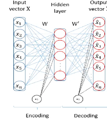
3.3.2. Autoencoder neural network... 46
3.4. Experimental Results... 48
3.4.1. Dataset Description and Experimental Setup... 48
3.4.2. Results and Discussion... 49
3.4.2.1 Results of the Convolutional Neural Networks based Method... 49
3.4.2.2 Results of the Autoencoder Neural Networks based Method... 51
3.5 Conclusion... 56
3.6. References... 57
Chapter 4. Multilabel Conditional Random Field Classification 4.1. Introduction ... 60
4.2. Proposed Method... 62
4.2.1. Monolabel Classification with CRF... 62
4.2.2. CRF for Multilabel Classification... 63
4.3. Experimental Validation... 66
4.3.1. Dataset Description and Experimental Setup... 66
4.4. Conclusion... 71
4.5. References... 71
Chapter 5. Spatial and Structured SVM for Multilabel Image Classification 5.1. Introduction ... 74
5.2. Problem Formulation and Tools... 77
5.2.1 Multilabel Classification for EHR Imagery... 77
5.2.2 Tile Representation... 78
5.2.3 Reviews of Structured SVM... 79
5.2.3. Structured SVM with Spatial Embedding... 81
5.3. Experimental Results... 84
5.3.1. Dataset Description... 84
5.3.2. Experimental Setup... 85
5.3.3. Experimental Results... 86
5.3.3.1 Results of Dataset... 86
5.3.3.2. Results of Dataset... 90
5.4. Conclusion... 93
5.5. References... 94
Chapter 6. Conclusions... 98
List of Tables:
Table 2.1. HMM notations in accordance to our detection problem. Table 2.2. General description of experiments conducted.
Table 2.3. Classification results for the first dataset (Experiments 1 - 3).
Table 2.4. Classification results for the second dataset at resolution of 224x224 (Experiment 4).
Table 2.5. Classification results for the second dataset at 640x480 and 1280x720 resolutions (Experiments 5 and 6).
Table 2.6. Classification results for the second dataset at 1920x1080 and 3840x2160 resolutions (Experiments 7 and 8).
Table 2.7. State transition matrix.
Table 2.8. HMM detection result at resolution of 244x224. Table 2.9. HMM detection results at VGA and 720p resolutions. Table 2.10. HMM detection results at 1080p and 4K resolutions.
Table 2.11. Detection speed (number of frames per second) for the second dataset.
Table 3.1. Comparison of classification accuracies in terms of sensitivity (SENS) and specificity (SPEC) between the different implementations. Computational time per tile is also reported for each strategy.
Table 3.2. Best threshold values yielded by the Otsu’s method for each of the RBFNN output classes.
Table 3.3. Comparison of classification accuracies in terms of sensitivity (SENS) and specificity (SPEC) between the different implementations. Computational time per tile is also reported for each strategy.
Table 3.4. Best threshold values yielded by the Otsu’s method for each of the AE-MLP based output classes.
Table 3.5. Sensitivity (SENS) and specificity (SPEC) accuracy achieved for each class by the reference method , the CNN-RBFNN and WAV-BOW with and without the multilabeling layer (ML) classifiers on dataset 1 (Povo).
Table 3.6. Sensitivity (SENS) and specificity (SPEC) accuracy achieved for each class by the reference method, the CNN-RBFNN and RGB-BOW with and without the multilabeling layer (ML) classifiers on dataset 1 (Civezzano).
Table 4.1. Sensitivity (SENS), specificity (SPEC) and average (AVG) accuracies in percent obtained by the different classification methods on datasets 1 and 2.
Table 4.2. class-by-class accuracy performances achieved by the three models on dataset 1 (Civezzano).
Table 4.3. class-by-class accuracy performances achieved by the three models on dataset 2(Munich).
Table 5.2. Number of class occurrence on dataset 2 (Munich).
Table 5.3. Classification accuracies of the three classifiers on dataset 1 (Civezzano).
Table 5.4. Statistical comparison based on MCNEMAR’s test between the three models on dataset 1 (Civezzano).
Table 5.5. Classification accuracies of the three classifiers on dataset 2 (Munich).
Table 5.6. Statistical comparison based on MCNEMAR’s test between the three models on dataset 2 (Munich).
Table 5.7. class-by-class accuracy performances achieved by the three models on dataset 1 (Civezzano).
Table 5.8. class-by-class accuracy performances achieved by the three models on dataset 2 (Munich).
List of Figures:
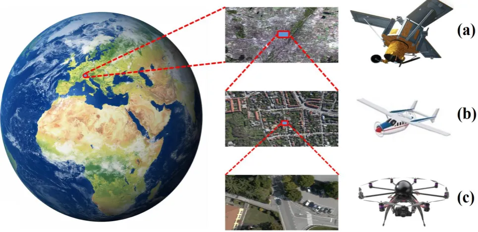
Fig. 1.1. Example of imagery spatial resolution differences of three acquisition platforms covering the same area.
(a) Satellite; (b) Airborne; (c) Unmanned aerial vehicle.
Fig. 1.2. Example of unmanned aerial vehicles usages in different application environments. Fig. 2.1. Block diagram of the overall system.
Fig. 2.2. Example of CNN architecture for object recognition.
Fig. 2.3. An example of operation performed by the neurons at a spatial location of the input and the resulting activation maps.
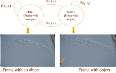
Fig. 2.4. State transition diagram (object pointed by a yellow arrow is a jacket used to simulate top half of buried victim).
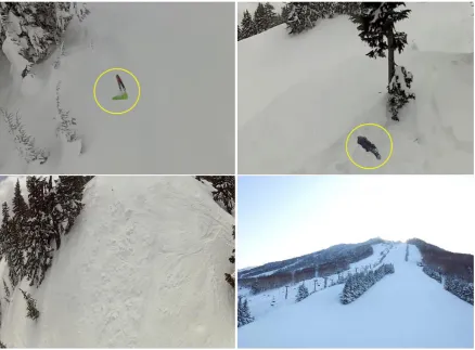
Fig. 2.5. Example of positive (top) and negative (bottom) images from the first dataset. Objects of interest (partially buried skis (left) and top half buried victim (right)) are marked with yellow circle.
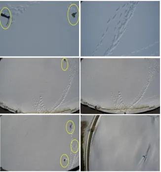
Fig. 2.6. Positive (left) and negative (right) frame snapshots from the second dataset. Objects of interest (skis, jacket to simulate bottom half buried victim, and ski pole) are marked by yellow circle.
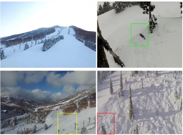
Fig. 2.7. Example of correctly classified negative (top left) and positive (top right), false positive object marked in yellow rectangle (bottom left), and false negative object marked by red rectangle (bottom right).
Fig. 2.8. Example showing the pre-processing step. The image on top shows a frame being scanned by a sliding window while the image on the bottom highlights a region (marked by blue rectangle), centered around a window (marked by cyan rectangle) selected for further processing.
Fig. 2.9. Snapshot of frames with correct positive (left) and negative (right) detection results at the VGA resolution from the second dataset. Regions of a frame containing an object are shown with green rectangle.
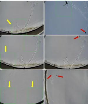
Fig. 2.10. Examples of false positive (left) and false negative (right) frame snapshots at VGA resolution. Yellow arrows indicate false positive regions in a frame whereas red arrows show missed objects in a frame.
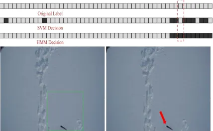
Fig. 2.11. Example of positive change by HMM. Sequence of white and black squares on top indicate label of successive frames. White square indicates a frame has object of interest whereas black square indicates the opposite. The frame where the change happened is highlighted by red dotted rectangle and the corresponding frame in the bottom. The frame for which SVM made wrong decision is shown in bottom left (the object in the frame, skis in this case, is indicated by red arrow) whereas the same frame corrected by HMM is shown in the bottom right (the object in the frame is indicated by green arrow). Note that object is not localized since post-processing decision is made at the frame level.
highlighted by red dotted rectangle. The frame for which SVM made the right decision, with the object localized in a green rectangle, is shown in the bottom left. The same frame for which HMM made wrong decision is shown in bottom right.
Fig. 2.13 Bar graph showing the change in accuracy and detection rate as resolution increases.
Fig. 3.1. Flow chart of the multilabel coarse classification framework. Fig. 3.2. Flow chart of the Inception module.
Fig. 3.3. Global flowchart of the proposed classification scheme.
Fig. 3.4. Graphical histogram illustration of the OTSU thresholding technique.
Fig. 3.5. Flow chart of the multilabel classification method based on the autoencoder network.
Fig. 3.6. Architecture of an AE network.
Fig. 3.7. The effect of the encoding rate on the average accuracy for (a) dataset 1 (Povo) and (b) dataset 2 (Civezzano).
Fig. 3.8. Example of two MLP output histograms and their decision threshold computed using OTSU’s method for WAV-AE,(a) class Asphalt, (b) class Grass in dataset one (Povo). Fig. 3.9-1 Qualitative map results of the 13 object classes obtained by the coarse WAV-AE (ML) classification technique on one of the test images of dataset 1(Povo) along with its related ground truth and original image.
Fig. 3.9-2 Qualitative map results of the 13 object classes obtained by the coarse GoogLeNet-RBFNN (ML) classification technique on one of the test images of dataset 1(Povo) along with its related ground truth and original image.
Fig. 3.9-3 Qualitative map results of the 14 object classes obtained by the coarse Alex-RBFNN (ML) classification technique on one of the test images of dataset 2 (Civezzano) along with its related ground truth and original image.
Fig. 4.1. Flow chart of the multilabel classification method
Fig. 4.2. The correlation and traditional spatial neighboring information in the proposed ML-CRF.
Fig. 4.3. Average accuracy versus spatial parameters 𝜆1, 𝜆2 achieved by the Full-ML-CRF
method on (a) dataset 1 (Civezzano) and (b) dataset 2 (Munich).
Fig. 4.4. Examples of multilabel classification maps obtained by the three classification methods (ML-Unary, ML-CRF, Full-ML-CRF) on two test images of dataset 2(Civezzano), along with their related ground truth and original image.
Fig.5.1. General block diagram of the proposed framework for multilabel tile-wise description.
Fig. 5.2. Output graph structure obtained for dataset 1 (Civezzano).
Fig. 5.4. (a) Ground truth of a test image of dataset 1 (Civezzano). (b, c, d) Classification results of the test image obtained by SVM(b), SSVM(c) and SSSVM(d). Each tile is colored according to the Hamming distance between the ground truth and prediction.
Fig. 5.5. Multilabel classification map obtained by the SSSVM classifier on one of the test images of dataset 1 (Civezzano), along with its related ground truth and original image. Fig. 5.6. Output graph structure obtained for dataset 2 (Munich).
Fig. 5.7. Average accuracy versus spatial parameter 𝝀 (of SSSVM model) for dataset 1 (Civezzano) (a) and dataset 2 (Munich) (b).
Fig. 5.8. (a) Ground truth of a test image of dataset 2 (Munich). (b, c, d) Classification results of the test image obtained by SVM(b), SSVM(c) and SSSVM(d). Each tile is colored according to the Hamming distance between the ground truth and prediction.
Glossary:
UAV: unmanned aerial vehicle
VHR: very high resolution
EHR: extremely high resolution
ANN: artificial neural network
CNN: convolutional neural network
RGB: red, green, blue
SVM: support vector machine
HMM: hidden markov models
HOG: histogram of oriented gradients
RBFNN: radial basis function neural network
MLP: multilayer perceptron network
SAR: synthetic aperture radar
LIDAR: light detection and ranging
AE:autoencoder network
OTSU:Otsu’s thresholding method
WAV:wavelets transform
BOW: bag of visual words
SENS: sensitivity
SPEC: specificity
AVG: average
SSVM: structured support vector machine
SSSVM: spatial and structured support vector machine
MRF: Markov random field
CRF: conditional random field
ML-CRF: multilabel conditional random field
Full-ML-CRF: full multilabel conditional random field
GAN: generative adversarial network
1
Chapter I
2
1.1. Remote Sensing Platforms and Applications
There exist several definitions for Remote Sensing; all of those definitions in the widest sense are concerned with information acquisition and measuring the reflected energy of areas and objects under monitoring without a direct contact. Remote Sensing can be divided into two categories, active and passive. Active remote sensing is when a signal is first emitted then the resulting reflected energy is analyzed. Active image sensors such as, satellites- and aircraft-based sensors emit their own energy (radiation pulse) which is transmitted to the object (i.e., earth surface) creating a backscatter that bounces and returns back to the emitting sensors again. This technique has shown great potential in collecting data whenever it is needed, day or night, without any time or atmospheric constraints, however it is energy demanding. Two common examples among the variety of existing active sensors that are widely used within the remote sensing community are Radars, and light detection and ranging (LiDAR). Radar and LiDAR are respectively, radio waves- and laser- based sensors used to collect information about the target under surveillance, such as distance, range, velocity, angle, and elevation. On the other hand, passive remote sensing simply acquires information using the energy that the target reflects (i.e., the sun, electromagnetic energy). It exploits the targets’ own energy, which is not energy demanding but depends on the external sources.
Over the last few decades, satellites have reached a good level of technological progress in terms of spatial resolution (i.e. Landsat 8 with 15 meters of spatial resolution). Such acquired information from satellites have been used widely, and showed to be efficient in various applications such as (e.g., forestry, cartography, forestry, climate, geology) [1]. However since the lunch of IKONOS the first very high resolution (VHR) optical satellite with (82-centimeter resolution and multispectral imagery of 4 meters), and then the last generation of VHR (i.e.,
Fig. 1.1. Example of imagery spatial resolution differences of three acquisition platforms covering the same area. (a) Satellite; (b) Airborne; (c) Unmanned aerial vehicle.
3
GeoEye-1 -2, QuickBird, WorldView-1 -2 & 3) a new level of spatial complexity has been exposed.
In particular, very high-resolution (VHR) satellites imagery has shown a remarkable performance and efficiency in several applications. For instance, in [2], using Multitemporal High-Resolution IKONOS and GeoEye-1 Satellites data, authors proposed a segmentation-based method exploiting support vector machines (SVMs) classifier to map urban ecological conditions, and to determine land cover changes in a dense urban core from 2000 to 2009. In [3], was presented an identification method for archaeological buried remains within a dense presence of vegetation using VHR Quickbird satellite data. In [4], authors introduced a bayesian classification framework of urban land use. It incorporates its open source data from very high resolution (VHR) GeoEye stereo satellite imagery. In [5], the authors presented an automatic moving vehicles information extraction framework from Single-Pass WorldView-2 VHR Imagery.
Similarly, airborne technologies equipped with VHR SAR and LiDAR sensors such as, helicopters, fixed wing aircrafts and single-rotor helicopters have shown to be very suitable for several urban landscape 3D modeling gaining a rapid growth in recent years. For instance, in [6], authors present a three dimensional reconstruction method for large multilayer interchange bridges using airborne light detection and ranging (LiDAR) data. In [7], authors put forth an image reconstruction algorithm for airborne downward-looking sparse linear array 3-D synthetic aperture radar (DLSLA 3-D SAR). Another Airborne LiDAR application for large urban environments was introduced in [8], particularly, a multiscale grid algorithm for the detection and reconstruction of building roofs. It derives benefits from making use of an iterative morphological interpolation exploiting a gradually increasing scale from large to small scales. Afterwards, the resulting building roofs features are segmented and reconstructed according to their elevation. In [9], it was introduced a woodland canopy reconstruction framework of digital terrain model (DTM) from an airborne E-SAR sensor. Another very interesting work has been presented in [10], where Paris et al. proposed a 3-dimentional model-based algorithm for tree top height estimation for high-spatial-density LiDAR data.
Notably, airborne sensors have proven to be very efficient in providing color/ infrared very high-resolution imagery. Outfitted with different sensors and technologies (i.e., camera, LIDAR), they are capable to acquire very accurate and high quality geometrical data of the observed areas. On the contrary, satellites imagery have a smaller resolution capability compared to airborne sensors. However, their coverage capacity is extremely large due to their very high altitude, saving the mosaicking and geocoding process that is required for aerial photography platforms when the scanned area is large (Fig. 1.1). Yet, satellites suffer from (i) cloud cover and (ii) specific fixed-timing acquisitions. As a result, airborne platforms are emerging as a potential strong alternative to conventional satellites acquisition technologies in both spectrally and spatially very high-resolution remote sensing imagery. Despite the afforested, airborne high cost and complicated flight procedures, in addition of their limited flight altitude, make of them a less appropriate acquisition platform for critical applications such as routine maintenance and emergency response.
4
characterized by low-cost, fast deployment and custom-made capacity, since they can be equipped with appropriate sensors according to the requirements of several distinct missions. Moreover, they play a complementary role in supporting satellites to cover inaccessible small areas, by taking advantage of their very detailed scanning capability at a sub meter / centimeter level i.e., extremely high image spatial resolution (EHR). Furthermore, UAVs grant the flexibility to operate within a swarm forming a complex acrobatic group flights that communicate and cooperate synchronously in mid-air. As to cope with their limited coverage scale, UAVs collect data in a timely manner providing a wider coverage capacity. Thanks to their smaller size and easier air traffic management compared to airborne platforms, UAVs stand out to be a favorable alternative to the traditional
field visit and ground surveying, and a very suitable acquisition platform to collect extremely high-resolution (EHR) data for several image classification and analysis applications such as, urban and environmental monitoring, precision farming, surveillance, and search and rescue missions (Fig. 1.2).
For instance, in mapping and cartography applications, Márquez et al. in [11], presented a framework that generates cadastral cartography for small urban/rural locations taking as input unmmaned aerial vehicles imagery. Pattern recognition algorithms were applied to add pictorial terrain components in the resulting cadastral plans. In [12], it was proposed a 3-D mapping system via a UAV flying from low altitude equipped with cameras, a laser scanner, an inertial measurement unit, and Global Positioning System (GPS). In [13], authors presented a novel range-dependent map-drift algorithm (RDMDA) developed for synthetic aperture radar (SAR) systems mounted on unmanned aerial vehicles (UAVs). One more interesting work in [14] put forth a stereo vision path planning assistant system for unmanned ground vehicle (UGV) in GPS-denied environments based on multiunmanned aerial vehicles. As for the inspection and public safety applications, a notable interest has been dedicated to UAVs platforms. In [15], a navigation prototype is developed to localize drone positions in indoor environments for industrial applications. Another automatic UAV inspection system is presented in [16]. This platform aims towards resource assessment and defect detection in large-scale photovoltaic systems over large geographical areas. Furthermore, in [17], Pinto et al. introduced an online inspection video monitoring system for industrial installations based on areial collaborative communications between small UAVs (i.e., UAV-to-UAV network). Concerning public safety, UAV aerial support provides a very adequate system to acquire information in unreachable areas. Aside from guaranteeing the safety of human operators from direct contact with danger in emergency
Fig. 1.2. Example of unmanned aerial vehicles usages in different application environments.
5
situations. For instance, [18] presented an autonomous UAV system equipped with thermal and digital imagery sensors for human body detection in disaster scenarios. The detected victim positions are geo-located within a map of points and then sent to the rescuing teams. [19] put forth a 3D UAV-based modeling for collapsed buildings rapid response situations in urban scenes. In [20], a semi-autonomous indoor fire-fighting to ensure firefighters safety is presented. Other works based on UAVs dealing with emergency and disaster fast response can be found in [21]-[22].
Moreover, UAVs have been finding their way in precision agricultural applications. By incorporating thermal, near-infrared and visible spectral bands to UAVs platform sensors, they serve as an alternative to traditional field visits to measure vegetation, health condition, and water stress indices, especially for large farmlands surveying. For instance, in [23] Katsigiannis et al. presented an autonomous multi-sensor UAV system that provides spectral information related to water management for pomegranate orchards. In [24], authors put forth a low cost multi-spectral vegetation classification platform of UAVs equipped with a set of exchangeable filters over a camera connected to a Raspberry Pi. The implemented prototype have shown to be able to distinguish between two types of vineyards and different species of plants. Authors in [25], presented a row and water front detection architecture combining UAV and thermal-infrared imagery for furrow irrigation monitoring. Still in precision farming, an interesting UAV-based network system for early stage disease detection was presented in [26]. In [27], authors presented an autonomous timely monitoring method for close range UAV citrus greening disease detection. It exploits depth-invariant machine learning models to distinguish between healthy and infected plant leaves. Very promising results have been yielded with validation accuracies up to 93%. Furthermore, plenty of other works involving UAVs have been undertaken in a wide range of areas, including but not limited to archaeology [28], radiation monitoring [29], ecological protection [30], and environmental monitoring in general [31],[32]. For further potential remote sensing applications of UAVs, we refer the reader to relevant state of the art.
1.2. Issues, Solutions and Thesis Organization
As with the evolution of UAVs technology which has known a dramatic increase for civilian applications over the last decade. UAVs have displayed a remarkable efficiency as a safer and job faster alternative to traditional field visit and ground surveying in urban scenarios. Such acquisition systems, despite their effectiveness, convey an extremely high-resolution (EHR) images with a very accurate geometrical analysis for the objects present in the scene, entailing a challenging huge amount of details to be processed and exploited (i.e., hundreds of spectral bands). This calls for the need to adopt new processing and analysis techniques that are capable to exploit the full potential of this huge amount of acquired information. Thus acquiring some main points to be dealt with, like:
6
large amount of details of the extremely high resolution data. Indeed, most of the monolabel processing methods have been applied successfully within constrained environments with moderate resolutions and a limited number of classes of objects to be predicted. This calls for the need to design new processing methods suggesting the use of multilabeling approaches.
The second one is that the objects in EHR imagery manifest two particular topologies of correlation, which could be exploited to enhance the recognition process. They are: i) the intrinsic correlation between objects (i.e., when a particular object is present, it is likely that another is present as well); ii) the spatial correlation between adjacent decisions, which may be provided by a given classifier.
Third, as a matter of fact, most UAV-oriented applications require real-time processing overhead. Therefore, the respective processing algorithms are ought to be implemented to meet such requirement.
1.3. Multilabel Classification
As hinted earlier, usually imagery analysis and classification applications for data acquired over urban areas are composed by a list of objects, that when are put together they describe the conventional scene. In order to address this, we extend the interest into describing several classes at the same time. Therefore, multilabel approach presents an alternative to the single object description making the classification task more informative and generalized.
In particular, the scope of this dissertation is mainly focused on describing extremely high resolution images in urban scenarios. Consequently, we dedicated three chapters to deal with multilabel classification, which is a subject that has attracted a scarce attention with respect to monolabel (i.e., binary and multiclass) classification. In fact, most of the processing methods and frameworks based on statistical modeling are mainly designed for monolabel tasks. Particularly, within the remote sensing community, monolabel classification and object detection has drawn the attention of most of researchers generating the largest number of published papers. In contrast to multiclass classification where the labels are mutually exclusive (only one object class per sample), multilabel classification associates to a single sample one or more than one label simultaneously (i.e., a list of object classes). As a result, as the number of classes exponentially increases, so does the classification output space complexity. A common way to address the multilabel issue, is to handle each class separately (i.e., in a class specific manner) then the resulting output of all the classes together is the final outcome. Such approach is very time consuming due to the number of algorithms (i.e., classifiers) that would be called simultaneously. Another critical point to be highlighted in multilabel classification is the inter-class correlation information between labels and how to exploit them effectively through the classification process. Therefore, we will try to benefit from handling all the object classes together rather than separately in order to extract some interaction rules between labels.
7
consideration the capability of the proposed approach in terms of its ability to resolve both the multilabel classification and the EHR spectral feature complexities characterizing this task.
In this respect, having devoted this first chapter as an introductive part to cover the different aspects of the topic. The rest of the thesis is organized into five chapters, in which the next chapter presents an interesting public safety application, namely, a framework based on UAV imagery for assisting avalanche search and rescue operations, whereas in the remaining three chapters, we put forth three proposed multilabeling classification schemes in urban scenarios. In more details, in Chapter 2, we put forth a victim detection and localization framework to assist rescue teams in avalanche search and rescue (SAR) operations my means of a UAV equipped with digital cameras. The proposed framework consists of three steps, 1) a pre-processing step to select regions of interest within the acquired images. 2) we use convolutional neural networks (CNN) for feature extraction and a Support Vector Machine (SVM) on top of it for classification. 3) a post-processing step based on a Hidden Markov Model is used to improve the prediction output of the SVM classifier.
In Chapter 3, we propose a tile-based pipeline that takes advantage of a tile-based coarse description technique providing global results for the considered EHR images. Considering the conventional pixel-based and segment-based descriptors that may raise the problem of intra-class variability particularly when dealing with the multilabel object detection. Coarse description strategy does not aim to assign to each single pixel or pattern descriptor a label, but it simply describes a query image or the specific investigated tile within the image by the list of objects present in it. In this context, two Deep Neural Networks (DNNs) architectures have been investigated namely, convolutional neural networks [33], and autoencoders [34] which have become one of the most promising and fast growing techniques within the machine learning community in the last few years. Moreover, for the multilabeling requirements, we introduce a multilabel layer that has been integrated on top of the proposed architectures to increase the obtained results.
8
techniques, which typically perform the multilabel classification task by separating the spectral features and the spatial contextual information into two different processing methods. We propose here a completely different alternative scheme called Spatial and Structured Support Vector Machine (SSSVM). Aiming at expanding the coarse tile-based multilabel spectral features classification scheme to incorporate the spatial information within the recognition process, we propose to merge both information, spectral and contextual within the same cost function. The resulting framework operates as an extension to the conventional Structured Support Vector Machine (SSVM) by integrating the structured output of the SVM and the spatial information simultaneously during the training phase. Finally, Chapter 6 draws final conclusions of the discussed methods and put forward some open issues and potential ameliorations for future developments.
This dissertation has been written supposing that the Reader is familiar with the basic concepts regarding the image processing, remote sensing and pattern recognition fields. Otherwise, the Reader is recommended to consult the references which are available at the end of each chapter of this dissertation. They are useful to give a complete and well-structured overview about the topics discussed throughout the manuscript. The following chapters have been written in such a way to be independent between each other to give to the Readers the possibility to read only the chapter/s of interest, without loss of information.
1.4. REFERENCES
[1] M. A. Wulder, J. C. White, S. N. Goward, J. G. Masek, J. R. Irons, M. Herold, W. B. Cohen, T. R. Loveland and C. E. Woodcock, “Landsat continuity: Issues and opportunities for land cover monitoring,” Remote Sensing of Environment, vol. 112, no. 3, pp. 955-969, 2008.
[2] J. Haas and Y. Ban, "Mapping and Monitoring Urban Ecosystem Services Using Multitemporal High-Resolution Satellite Data," in IEEE Journal of Selected Topics in Applied Earth Observations and Remote Sensing, vol. 10, no. 2, pp. 669-680, Feb. 2017.
[3] R. Lasaponara and N. Masini, "Identification of archaeological buried remains based on the normalized difference vegetation index (NDVI) from Quickbird satellite data," in IEEE Geoscience and Remote Sensing Letters, vol. 3, no. 3, pp. 325-328, July 2006.
[4] M. Li, K. M. de Beurs, A. Stein and W. Bijker, "Incorporating Open Source Data for Bayesian Classification of Urban Land Use From VHR Stereo Images," in IEEE Journal of Selected Topics in Applied Earth Observations and Remote Sensing, vol. PP, no. 99, pp. 1-14.
[5] B. Salehi, Y. Zhang and M. Zhong, "Automatic Moving Vehicles Information Extraction From Single-Pass WorldView-2 Imagery," in IEEE Journal of Selected Topics in Applied Earth Observations and Remote Sensing, vol. 5, no. 1, pp. 135-145, Feb. 2012.
[6] L. Cheng, Y. Wu, Y. Wang, L. Zhong, Y. Chen and M. Li, "Three-Dimensional Reconstruction of Large Multilayer Interchange Bridge Using Airborne LiDAR Data," in IEEE Journal of Selected Topics in Applied Earth Observations and Remote Sensing, vol. 8, no. 2, pp. 691-708, Feb. 2015.
9
[8] Y. Chen, L. Cheng, M. Li, J. Wang, L. Tong and K. Yang, "Multiscale Grid Method for Detection and Reconstruction of Building Roofs from Airborne LiDAR Data," in IEEE Journal of Selected Topics in Applied Earth Observations and Remote Sensing, vol. 7, no. 10, pp. 4081-4094, Oct. 2014.
[9] C. S. Rowland and H. Balzter, "Data Fusion for Reconstruction of a DTM, Under a Woodland Canopy, From Airborne L-band InSAR," in IEEE Transactions on Geoscience and Remote Sensing, vol. 45, no. 5, pp. 1154-1163, May 2007.
[10] C. Paris and L. Bruzzone, "A Three-Dimensional Model-Based Approach to the Estimation of the Tree Top Height by Fusing Low-Density LiDAR Data and Very High Resolution Optical Images," in IEEE Transactions on Geoscience and Remote Sensing, vol. 53, no. 1, pp. 467-480, Jan. 2015.
[11] E. S. Márquez and A. V. Soto, "Cadastral stereo plotting production from unmmaned aerial vehicles imagery," 2017 First IEEE International Symposium of Geoscience and Remote Sensing (GRSS-CHILE), Valdivia, 2017, pp. 1-9.
[12] M. Nagai, T. Chen, R. Shibasaki, H. Kumagai and A. Ahmed, "UAV-Borne 3-D Mapping System by Multisensor Integration," in IEEE Transactions on Geoscience and Remote Sensing, vol. 47, no. 3, pp. 701-708, March 2009.
[13] L. Zhang, M. Hu, G. Wang and H. Wang, "Range-Dependent Map-Drift Algorithm for Focusing UAV SAR Imagery," in IEEE Geoscience and Remote Sensing Letters, vol. 13, no. 8, pp. 1158-1162, Aug. 2016.
[14] J. H. Kim, J. w. Kwon and J. Seo, "Multi-UAV-based stereo vision system without GPS for ground obstacle mapping to assist path planning of UGV," in Electronics Letters, vol. 50, no. 20, pp. 1431-1432, September 25 2014.
[15] K. J. Wu, T. S. Gregory, J. Moore, B. Hooper, D. Lewis and Z. T. H. Tse, "Development of an indoor guidance system for unmanned aerial vehicles with power industry applications," in IET Radar, Sonar & Navigation, vol. 11, no. 1, pp. 212-218, 1 2017.
[16] X. Li, Q. Yang, Z. Chen, X. Luo and W. Yan, "Visible defects detection based on UAV-based inspection in large-scale photovoltaic systems," in IET Renewable Power Generation, vol. 11, no. 10, pp. 1234-1244, 8 16 2017.
[17] L. R. Pinto, A. Moreira, L. Almeida and A. Rowe, "Characterizing Multihop Aerial Networks of COTS Multirotors," in IEEE Transactions on Industrial Informatics, vol. 13, no. 2, pp. 898-906, April 2017.
[18] P. Rudol and P. Doherty, "Human Body Detection and Geolocalization for UAV Search and Rescue Missions Using Color and Thermal Imagery," 2008 IEEE Aerospace Conference, Big Sky, MT, 2008, pp. 1-8.
[19] S. Verykokou, A. Doulamis, G. Athanasiou, C. Ioannidis and A. Amditis, "UAV-based 3D modelling of disaster scenes for Urban Search and Rescue," 2016 IEEE International Conference on Imaging Systems and Techniques (IST), Chania, 2016, pp. 106-111.
[20] A. Imdoukh, A. Shaker, A. Al-Toukhy, D. Kablaoui and M. El-Abd, "Semi-autonomous indoor firefighting UAV," 2017 18th International Conference on Advanced Robotics (ICAR), Hong Kong, 2017, pp. 310-315.
10
[22] C. Corrado and K. Panetta, "Data fusion and unmanned aerial vehicles (UAVs) for first responders," 2017 IEEE International Symposium on Technologies for Homeland Security (HST), Waltham, MA, 2017, pp. 1-6.
[23] P. Katsigiannis, L. Misopolinos, V. Liakopoulos, T. K. Alexandridis and G. Zalidis, "An
autonomous multi-sensor UAV system for reduced-input precision agriculture
applications," 2016 24th Mediterranean Conference on Control and Automation (MED), Athens, 2016, pp. 60-64.
[24] J. Natividade, J. Prado and L. Marques, "Low-cost multi-spectral vegetation classification using an Unmanned Aerial Vehicle," 2017 IEEE International Conference on Autonomous Robot Systems and Competitions (ICARSC), Coimbra, 2017, pp. 336-342.
[25] D. Long, C. McCarthy and T. Jensen, "Row and water front detection from UAV thermal-infrared imagery for furrow irrigation monitoring," 2016 IEEE International Conference on Advanced Intelligent Mechatronics (AIM), Banff, AB, 2016, pp. 300-305.
[26] P. Menendez-Aponte, C. Garcia, D. Freese, S. Defterli and Y. Xu, "Software and Hardware Architectures in Cooperative Aerial and Ground Robots for Agricultural Disease Detection," 2016 International Conference on Collaboration Technologies and Systems (CTS), Orlando, FL, 2016, pp. 354-358.
[27] S. K. Sarkar, J. Das, R. Ehsani and V. Kumar, "Towards autonomous phytopathology: Outcomes and challenges of citrus greening disease detection through close-range remote sensing," 2016 IEEE International Conference on Robotics and Automation (ICRA), Stockholm, 2016, pp. 5143-5148.
[28] R. Saleri et al., "UAV photogrammetry for archaeological survey: The Theaters area of Pompeii," 2013 Digital Heritage International Congress (DigitalHeritage), Marseille, 2013, pp. 497-502.
[29] G. V. Prado and M. A. Y. Medina, "Design and Implementation of a Non-ionizing Radiation Measuring System Evaluated with an Unmanned Aerial Vehicle," 2015 Asia-Pacific Conference on Computer Aided System Engineering, Quito, 2015, pp. 52-57.
[30] N. Li, D. Zhou, F. Duan, S. Wang and Y. Cui, "Application of unmanned airship image system and processing techniques for identifying of fresh water wetlands at a community scale," 2010 18th International Conference on Geoinformatics, Beijing, 2010, pp. 1-5.
[31] Y. Lu, D. Macias, Z. S. Dean, N. R. Kreger and P. K. Wong*, "A UAV-Mounted Whole Cell Biosensor System for Environmental Monitoring Applications," in IEEE Transactions on NanoBioscience, vol. 14, no. 8, pp. 811-817, Dec. 2015.
[32] R. Ke, S. Kim, Z. Li and Y. Wang, "Motion-vector clustering for traffic speed detection from UAV video," 2015 IEEE First International Smart Cities Conference (ISC2), Guadalajara, 2015, pp. 1-5.
[33] Y. Lecun, L. Bottou, Y. Bengio and P. Haffner, "Gradient-based learning applied to document recognition," in Proceedings of the IEEE, vol. 86, no. 11, pp. 2278-2324, Nov 1998.
11
Chapter II
12
Abstract– Following an avalanche, one of the factors that affect victims chance of survival is the speed at which they get located and dugout. Rescue teams use techniques like trained rescue dogs and electronic transceivers to locate victims. However, the amount of resource required and time to deploy rescue teams are major bottlenecks to increase victim’s chance of survival. Advances in the field of Unmanned Aerial Vehicles (UAVs) have enabled the use of flying robots equipped with sensors like optical cameras to assess damages caused by natural or manmade disasters and locate victims in the debris. In this chapter, we propose to assist avalanche search and rescue (SAR) operations with UAVs fitted with vision cameras. The sequence of images of the avalanche debris captured by the UAV is processed with a pre-trained Convolutional Neural Network (CNN) to extract discriminative features. A trained linear Support Vector Machine (SVM) is integrated at the top of the CNN to detect objects of interest. Moreover, we introduce a pre-processing method to increase the detection rate and a post-processing method based on a Hidden Markov Model to improve prediction performance of the classifier. Experimental results conducted on two different datasets at different levels of resolution show that detection performance increases with an increase in resolution while the computation time increases. Additionally, they also suggest that a significant decrease in processing time can be achieved thanks to the pre-processing step.
2.1. Introduction
An avalanche, a large mass of snow detached from a mountain slope and sliding suddenly downward, kills more than one hundred fifty people worldwide [1] every year. According to the Swiss institute for snow and avalanche research, more than 90 percent of avalanche fatalities are occurred in uncontrolled terrain, like for example during off-piste skiing and snowboarding, [2]. Backcountry avalanches are mostly triggered by skiers or snowmobilers. Though it is rare, they can also be triggered naturally due to an increased load from a snow fall, metamorphic changes in snow pack, rock fall, and icefall. The enormous amount of snow carried at a high speed can cause a significant destruction to life as well as property. In areas where avalanches pose significant threat to people and infrastructure, preventive measures like snow fences, artificial barriers and explosives, to dispose avalanche potential snow packs, are taken to prevent and lessen their obstruction power.
Several factors account for the victims’ survival. For example, victims can collide with obstacles while carried away by avalanches or fall over a cliff in the avalanches path and get physically injured. Once the avalanche stops, it settles like a rock and body movement is nearly impossible. Victims chance of survival depends on the degree of burial, presence of clear airway, and severity of physical injuries. Additionally, duration of burial is also a factor for victims’ survival. According to statistics, 93 percent of victims survive if dugout within fifteen minutes of complete burial. Survival chance drops fast after the first fifteen minutes of complete burial. A “complete burial” is defined as where snow covers victims’ head and chest; otherwise the term partial burial applies, [3]. Therefore, avalanche SAR operation is time critical.
13
transceivers are powered by batteries and require experience to use. RECCO rescue system is an alternative to transceivers where one or more passive reflectors are embedded into clothes, boots, helmets, etc. worn by skiers and a detector is used by rescuers to locate the victims. Once area of burial is identified, a probe can be used to localize the victim and estimate the depth of snow to be shoveled. Additionally, an organized probe line can also be used to locate victims not equipped with electronic transceivers or if locating with the transceivers fails. But such technique requires significant man power and is a slow process. Recent advances in the field of UAVs have enabled the use of flying robots equipped with ARVA transceivers and other sensors to assist post-avalanche SAR operations, [4–6]. This has allowed to reduce search time and to search in areas that are difficult to reach and dangerous for rescuers.
In the literature, there are active remote sensing methods proposed to assist post-avalanche SAR operation. For example, the authors in [7] have shown that it is possible to detect victims buried under snow by using a Ground Penetrating Radar (GPR). Since human body has a high dielectric permittivity relative to snow, a GPR can uniquely image human body buried under snow and differentiate it from other man-made and natural objects. With the advent of satellite navigational system, Jan S, et.al [8], studied the degree to which a GPS signal can penetrate through the snow and be detected by a commercial receiver, hence a potential additional tool for quick and precise localization of buried victims. Following the work in [8], the authors in [9] also studied the performance of low cost High Sensitivity GPS (HSGPS) receivers available in the market for use in post-avalanche SAR operation. In a more recent work, Victor et.al [10] studied the feasibility of 4G-LTE signals to assist SAR operations for avalanche buried victims and presented a proof of concept that using a small UAV equipped with sensors that can detect cellphone signals, it is possible to detect victim’s cellphone buried up to seven feet deep. Though there has been no research published documenting the use of vision based methods, a type of passive remote sensing methods, specifically for post-avalanche SAR operation, it is possible to find papers that propose to support SAR operations in general with image analysis techniques. Rudol et.al., [11], proposed to assist wilderness SAR operation with videos collected using a UAV with an onboard thermal and color cameras. In their experiment, the thermal image is used to find regions with possible human body and corresponding regions in the color image are further analyzed by an object detector that combines Haar feature extractor with cascade of boosted classifiers. Because of partial occlusion and variable pose of victims, the authors in [12] demonstrated models that decompose complex appearance of humans into multiple parts, [13–15], are more suited than monolithic models to detect victims laying on the ground from aerial images captured by UAV. Furthermore, they have also shown that integrating prior scale information from inertial sensors of the UAV helps to reduce false positives and a better performance can be obtained by combining complementary outputs of multiple detectors.
14
applications like post-avalanche SAR operation. According to [19] out of 1886 people by avalanche in Switzerland between 1981 and 1998, 39% of the victims were buried with no visible parts while the rest are partially buried or stayed completely unburied on the surface. Moreover, chance of complete burial can be reduced if avalanche balloons are used. With this statistics, we present a method that utilizes UAVs equipped with vision sensors to scan the avalanche debris and further process the acquired data with image processing techniques to detect avalanche victims and objects related to the victims in near-real time.
Organization of this chapter is as follows: the overall block diagram of the system along with the description of each block is presented in the next section. Datasets used and experimental setup are presented in section 3. Experimental results are presented in section 4 and the last section, section 5, is dedicated to conclusion and further development.
2.2. Methodology
In this section we present a pre-processing method, partially based on image segmentation technique, to filter areas of interest from a video frame followed by an image representation method based on Convolutional Neural Networks (CNNs or ConvNets) and train a Support Vector Machine (SVM) classifier to detect objects. Furthermore, we present a post-processing method based on Hidden Markov Models (HMMs) to take advantage of the correlation between successive video frames to improve decision of the classifier. Block diagram of the overall system is shown in Fig 2.1.
Fig. 2.1. Block diagram of the overall system
2.2.1. Pre-processing
15
pre-processing step, a frame will be scanned with a sliding window and each window will be checked for a color different than snow by thresholding saturation component of the window in the HSV color space. We have adopted the thresholding scheme proposed in [20]:
𝑡ℎ𝑠𝑎𝑡(𝑉) = 1.0 −0.8𝑉
255, (1)
where V represents the value of the intensity component. We decide that a pixel corresponds to an object if the value of the saturation component S is greater or equal than thsat(V). In such a case,
the window is said to contain an object.
2.2.2. Feature Extraction
Feature extraction is the process of mapping image pixels or groups of pixels into a suitable feature space. The choice of an appropriate feature extractor strongly affects the performance of the classifier. In the literature, one can find several feature extraction methods proposed for object detection in images or videos. Haar, Scale Invariant Feature Transform (SIFT), and Histogram of Gradients (HOG) are some of the most widely used methods to generate image descriptors. In recent years, the availability of large real world datasets like ImageNet [21] and high performance computing devices have enabled the capability to train deep and improved neural network architectures like ConvNets. These classifiers have significantly improved object detection and classification performances. Beside training CNNs to learn features for a classification task, using pre-trained CNN architectures as a generic feature extractor and training classifiers like SVM has outperformed the performance results obtained by using hand designed feature extractors like SIFT and HOG [22,23].
16
Fig. 2.2. Example of CNN architecture for object recognition
2.2.2.1. Convolutional Layer
The convolutional layer is the main building block of a ConvNet that contains a set of learnable filters. These filters are small spatially (along the height and width dimension) and extend fully in the depth dimension. Through training, the network learns these filters that activate neurons when they see a specific feature at a spatial position of the input. The convolution layer performs a 2-D convolution of the input with a filter and produce a 2-D output called activation map (Fig. 2.3). Several filters can be used in a single convolutional layer and the activation maps of each filter are stacked to form the output of this layer, which is an input to the next layer. The size of the output is controlled by three parameters: depth, stride, and zero padding. The depth parameter controls the number of filters in a convolutional layer. Stride is used to control the extent of overlap between adjacent receptive fields and has impact on the spatial dimension of the output volume. Zero padding is used to specify the number of zeros that need to be padded on the border of the input, which allows to preserve input spatial dimension at the output. Although there are other types of non-linear activation functions, such as the sigmoid and tanh , the most commonly used activation function in ConvNets is the rectified linear unit (ReLu) [25] that thresholds the input at zero. They are simple to implement and their non-saturating form accelerates the convergence of stochastic gradient descent [26].
17
2.2.2.2. Pooling Layer
In addition to weight sharing, CNNs use pooling layers to control overfitting. A pooling layer performs down sampling of the input in the spatial dimensions. Similar to convolutional layers, it also has stride and filter size parameters that control the spatial size of the output. Each element in the output activation map corresponds to the aggregate statistics of the input at the corresponding spatial position. In addition to control overfitting, pooling layers help to achieve spatial invariance [27]. The most commonly used pooling operations in CNNs are the max pooling, which computes maximum response of a given patch, the average pooling, which computes average response of a given patch, and the sub sampling (Equation 2) [27]
𝑎𝑗 = tanh(𝛽 ∑ 𝑎𝑖𝑛×𝑛
𝑁×𝑁
+ 𝑏) (2)
which computes the average over a patch of size 𝑛 × 𝑛, multiply it with a trainable parameter 𝛽, add a trainable bias 𝑏, and applies a non-linear function.
2.2.2.3. Fully Connected Layer
This layer is a regular multi-layer perceptron (MLP), where a neuron is connected to all neurons in the previous layer, that is used for classification. Once the network is setup the weights and biases are learned by using variants of the gradient descent algorithm. The algorithm requires to compute the derivative of a training loss with respect to the network parameters using the backpropagation algorithm. In the context of classification, the cross-entropy loss function is used in combination with the softmax classifier.
18
2.2.3. Classifier
The next step after feature extraction is to train a classifier suited for the task at hand. The choice of the classifier should take into account dimensionality of the feature space, the number of training samples available and any other requirements of the application. Motivated by their effectiveness in hyperdimensional classification problems, we will adopt the SVM classifier in this work. Introduced by Vapnik and Chervonenkis, SVMs are supervised learning models used to analyze data for classification and regression analysis. The main objective of such models is to find an optimal hyperplane or set of hyperplanes (in multiclass object discrimination problems) that separates a given dataset. They have been applied to a wide range of classification and regression tasks, [31–33].
Consider a binary classification problem with 𝑁 training samples in a 𝑑-dimensional feature space 𝑥𝑖𝜖ℜ𝑑(𝑖 = 1, 2, 3, … , 𝑁)with corresponding labels 𝑦𝑖𝜖{−1, +1}. There is an optimal hyperplane defined by a vector 𝑤𝜖ℜ𝑑 normal to the plane and a bias 𝑏𝜖ℜ that minimizes the cost function [34] given by:
𝜓(𝑤, 𝜉) =1 2‖𝑤‖
2
+ 𝐶 ∑ 𝜉𝑖
𝑁
𝑖=1
(3)
subject to the following constraints:
{𝑦𝑖(𝑤 ⋅ 𝜙(𝑥𝑖) + 𝑏) ≥ 1 − 𝜉𝑖, 𝑖 = 1,2,3, … , 𝑁
𝜉𝑖 ≥ 0, 𝑖 = 1,2,3, … , 𝑁 (4)
The cost function in equation 3 combines both margin maximization (separation between the two classes) and error minimization (penalizing wrongly classified samples) in order to account for non separability in real data. The slack variables (𝜉𝑖’s) are used to take into account non separable data while 𝐶 is a regularization parameter that allows to control the penalty assigned to errors. Though initially designed for linearly separable data, SVMs were later extended to nonlinear patterns by using kernel tricks. A kernel function aims at transforming the original data into a new higher dimensional space using kernel functions (𝜙(. )’s) and classification (or regression) is performed in the transformed space. Membership decision is made based on the sign of a discriminant function 𝑓(𝑥) associated with the hyperplane. Mathematically,
𝑦̂ = 𝑠𝑖𝑔𝑛{𝑓(𝑥)}, where
𝑓(𝑥) = 𝑤 ⋅ 𝜙(𝑥) + 𝑏,
19
2.2.4. Post-Processing
In a video sequence, it can be reasonably expected that the change in content of successive frames is small. Therefore, it is highly likely for an object to appear in consecutive frames. With this in mind, we propose to resort to hidden markov models to improve decision of the classifier for a frame at time 𝑡 based on the previous frame decisions. HMMs are statistical Markov models useful to characterize systems where unobserved internal state governs the external observations we make. They have been applied to a wide range of applications like human activity recognition from sequential images, bioinformatics, speech recognition, computational and molecular biology, etc., [35,36].
Consider a system with 𝑁 distinct states, 𝑆 = {𝑠1, 𝑠2, 𝑠3, … , 𝑠𝑁}, and 𝑀 distinct observation symbols, 𝑉 = {𝑣1, 𝑣2, 𝑣3, … , 𝑣𝑀}, per state. Given the following parameters,
1. State transition matrix, 𝐴 = [𝑎𝑖𝑗]: probability that the system will be in state 𝑠𝑗 at time 𝑡 given the previous state is 𝑠𝑖.
𝑎𝑖𝑗 = Pr(𝑞𝑡 = 𝑠𝑗|𝑞𝑡−1= 𝑠𝑖) , 1 ≤ 𝑖, 𝑗 ≤ 𝑁 (6)
where 𝑞𝑡 is the state at time t.
2. Initial state probability, 𝜋: state of the system at time 𝑡 = 0
𝜋 = Pr(𝑞0 = 𝑠𝑖) (7)
3. Observation symbol probability distribution in state 𝑠𝑗, 𝐵 = [𝑏𝑗(𝑘)] 𝑏𝑗(𝑘) = 𝑃𝑟(𝑥𝑡 = 𝑣𝑘|𝑞𝑡 = 𝑠𝑗) , 1 ≤ 𝑗 ≤ 𝑁
1 ≤ 𝑘 ≤ 𝑀 (8)
where 𝑥𝑡 is the observation at time 𝑡
and given also the two main HMM assumptions, i.e., first order Markov assumption (a state at time 𝑡 only depends on a state at time 𝑡 − 1) and the independence assumption (output observation at time 𝑡 is only dependent on a state at time 𝑡), there are three basic problems that need to be solved in the development of a HMM methodology. These are:
1) Evaluation problem: the objective of this problem is to calculate the probability of an observation sequence, 𝑂 = 𝑜1, 𝑜2, … , 𝑜𝑇, given model parameters 𝜆 = (𝐴, 𝐵, 𝜋), i.e.
𝑃(𝑂|𝜆). Besides, it can also be viewed as a way of evaluating how the model can predict the given observation sequence.
2) Decoding problem: it deals with finding the optimal state sequence, 𝑆 = 𝑠1, 𝑠2, … , 𝑠𝑇, that best explains a given observation sequence, 𝑂 = 𝑜1, 𝑜2, … , 𝑜𝑇, given model parameters 𝜆.
3) Learning problem: it consists in estimating model parameters, 𝜆 = (𝐴, 𝐵, 𝜋), from a given training data (supervised or unsupervised) to maximize 𝑃(𝑂|𝜆).
20 𝑞𝑡∗ = 𝑎𝑟𝑔𝑚𝑎𝑥
1≤𝑖≤2
𝑃(𝑞𝑡= 𝑠𝑖|𝑜1, 𝑜2, … , 𝑜𝑡, 𝜆) (9)
Table 2.1. HMM notations in accordance to our detection problem
𝑠1 𝑦 = ′ − 1′
𝑠2 𝑦 =′+ 1′
𝑜𝑡 𝑥𝑡 (image aquired at time t)
𝑦𝑡 𝑦̂ (equation 4)
The state diagram is shown in Fig. 2.4. There exists an efficient dynamic programming algorithm called the forward algorithm, [36], to compute the probabilities. The algorithm consists of the following two steps:
1. Prediction step: predict the current state given all the previous observations
𝑃(𝑞𝑡|𝑥𝑡−1, 𝑥𝑡−2, … , 𝑥1) = ∑ 𝑃(𝑞𝑡|𝑞𝑡−1)
𝑠𝑡−1
𝑃(𝑞𝑡−1|𝑥𝑡−1, 𝑥𝑡−2, … , 𝑥1) (10)
2. Update step: update the prediction based on the current observation
𝑃(𝑞𝑡|𝑥𝑡, 𝑥𝑡−1, … , 𝑥1) =
𝑃(𝑥𝑡|𝑞𝑡)𝑃(𝑞𝑡|𝑥𝑡−1, 𝑥𝑡−2, … , 𝑥1) ∑ 𝑃(𝑥𝑥𝑡 𝑡|𝑞𝑡)𝑃(𝑞𝑡|𝑥𝑡−1, 𝑥𝑡−2, … , 𝑥1)
(11)
using Bayes probability theorem
𝑃(𝑥𝑡|𝑞𝑡) =𝑃(𝑞𝑡|𝑥𝑡)𝑃(𝑥𝑡)
𝑃(𝑞𝑡) (12)
substituting equation 12 into 11, we obtain
𝑃(𝑞𝑡|𝑥𝑡, 𝑥𝑡−1, … , 𝑥1) = 𝑃(𝑞𝑡|𝑥𝑡)𝑃(𝑞𝑡|𝑥𝑡−1, 𝑥𝑡−2, … , 𝑥1)
21
Fig. 2.4. State transition diagram (object pointed by a yellow arrow is a jacket used to simulate top half of buried victim)
The posterior probability, 𝑃(𝑞𝑡|𝑥𝑡), is obtained by converting SVM classifier decision into a probability using the Platt scaling method, [37]. Platt scaling is a way of transforming outputs of a discriminative classification model (like SVM) into a probability distribution over the classes. Given a discriminant function,𝑓(𝑥), of a classifier, the method works by fitting a logistic regression model to the classifier scores. Mathematically,
𝑃(𝑦 = 1|𝑥) = 1
1 + 𝑒𝑥𝑝(𝐴𝑓(𝑥) + 𝐵) (14)
where the parameters 𝐴 and 𝐵 are fitted using the maximum likelihood estimation method from a training set by minimizing the cross-entropy error function.
2.3. Data and Experimental Setup
2.3.1. Dataset Description
22
Fig. 2.5. Example of positive (top) and negative (bottom) images from the first dataset. Objects of interest (partially buried skis (left) and top half buried victim (right)) are marked with yellow circle.
The second dataset is recorded on a mountain close to the city of Trento using a GoPro camera mounted on a CyberFed “Pinocchio” hexacopter. It consists of five videos of different durations recorded in 4K resolution (3840x2160) at a rate of 25 frames per second. For convenience, let us call each video as video 1, video 2…, up to video 5. Videos 1, 2, 3, and 4 are recorded at a height in the range of 2 to 10 meters while video 5 is recorded at a relatively higher height, which is between 20 and 40 meters. The first two videos were recorded with the camera at
23
Fig. 2.6. Positive (left) and negative (right) frame snapshots from the second dataset. Objects of interest (skis, jacket to simulate bottom half buried victim, and ski pole) are marked by yellow circle.
2.3.2. Setup
As explained earlier, since our dataset is small and objects of interest are among the thousand classes onto which GoogleNet is trained, we have used the network as a feature extractor. For this purpose, we removed the classification layer (layer 25) of the network. A forward propagation of zero center normalized image of size 224x224 through the network outputs a vector of image descriptor with 1024 elements.
Moreover, since processing time is critical to our problem and data is distributed in a high dimensional space, we train linear SVM for the task of classification. Both training and test features are scaled to have a unit length (equation 14) and the choice of best 𝐶 (regularization factor) is performed with a grid search of values in the range of 2−15 to 25 using two fold cross validation.
𝑥′= 𝑥
24
We have used the MatConvNet library [38] to operate on the pre-trained model and LibSVM library [39] to train SVM. All the experiments were conducted on a standard desktop computer with clock speed of 3GHz and 8GB RAM.
2.4. Results and Discussions
In this section, we report experimental results obtained for both datasets. General information about all experiments conducted can be found in Table 2.2. Accuracy, probability of true positives (𝑃𝑇𝑃), and probability of false alarm (𝑃𝐹𝐴) are the performance metrics used. 𝑃𝑇𝑃 and 𝑃𝐹𝐴 are calculated as follows:
𝑃𝑇𝑃 =
∑ #𝑜𝑓𝑝𝑜𝑠𝑖𝑡𝑖𝑣𝑒𝑠𝑎𝑚𝑝𝑙𝑒𝑠𝑐𝑜𝑟𝑟𝑒𝑐𝑡𝑙𝑦𝑐𝑙𝑎𝑠𝑠𝑖𝑓𝑖𝑒𝑑
∑ #𝑜𝑓𝑝𝑜𝑠𝑖𝑡𝑖𝑣𝑒𝑠𝑎𝑚𝑝𝑙𝑒𝑠 (16)
𝑃𝐹𝐴=
∑ #𝑜𝑓𝑛𝑒𝑔𝑎𝑡𝑖𝑣𝑒𝑠𝑎𝑚𝑝𝑙𝑒𝑠𝑐𝑙𝑎𝑠𝑠𝑖𝑓𝑖𝑒𝑑𝑎𝑠𝑝𝑜𝑠𝑖𝑡𝑖𝑣𝑒
∑ #𝑜𝑓𝑛𝑒𝑔𝑎𝑡𝑖𝑣𝑒𝑠𝑎𝑚𝑝𝑙𝑒𝑠 (17)
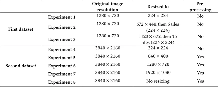
Table 2.2. General description of experiments conducted
Original image
resolution Resized to
Pre-processing
First dataset
Experiment 1 1280 × 720 224 × 224 No
Experiment 2 1280 × 720 672× 448, then6 tiles
(224 × 224)
No
Experiment 3 1280 × 720 1120× 672, then15
tiles (224 × 224)
No
Second dataset
Experiment 4 3840 × 2160 224 × 224 No
Experiment 5 3840 × 2160 640 × 480 Yes
Experiment 6 3840 × 2160 1280 × 720 Yes
Experiment 7 3840 × 2160 1920 × 1080 Yes
Experiment 8 3840 × 2160 No resizing Yes
2.4.1. Experiments without pre-processing
25
Table 2.3. Classification results for the first dataset (Experiments 1 - 3).
Accuracy (%) 𝑃𝑇𝑃 𝑃𝐹𝐴
Experiment 1 65.71 0.8462 0.5283
Experiment 2 94.29 0.6346 0.1095
Experiment 3 97.59 0.8065 0.0152
From Table 2.3, it is clear that the overall accuracy increases and 𝑃𝐹𝐴 decreases with an increase in resolution. Contrarily, 𝑃𝑇𝑃 decreases as for the second and third experiments with respect to the first and it increases for the third experiment with respect to the second. We believe that the reason for having a high 𝑃𝑇𝑃 in the first experiment is because we are considering the whole frame, which contains unwanted objects like poles, trees, lift lines, etc. In the first experiment we have high 𝑃𝐹𝐴 because the whole frame is resized to 224x224. The resizing makes objects of interest become insignificant with respect to the surrounding and thus forces the classifier to learn not only objects of interest but also the surrounding. On the other hand, second and third experiments have small
𝑃𝐹𝐴 and increased 𝑃𝑇𝑃 due to tiling, which makes objects of interest in a tile to become more significant with respect to the surrounding and the classifier is able to better discriminate objects of interest from the background. Some qualitative results are shown in Fig. 2.7.
Fig. 2.7. Example of correctly classified negative (top left) and positive (top right), false positive object marked in yellow rectangle (bottom left), and false negative object marked by red rectangle (bottom right).