R E S E A R C H
Open Access
Two-parameter regularization method for
an axisymmetric inverse heat problem
Ngo Van Hoa
1,2*and Tra Quoc Khanh
3*Correspondence:
[email protected] 1Division of Computational
Mathematics and Engineering, Institute for Computational Science, Ton Duc Thang University, Ho Chi Minh City, Vietnam
2Faculty of Mathematics and
Statistics, Ton Duc Thang University, Ho Chi Minh City, Vietnam Full list of author information is available at the end of the article
Abstract
In this paper we consider the inverse time problem for the axisymmetric heat equation which is a severely ill-posed problem. Using the modified quasi-boundary value (MQBV) method with two regularization parameters, one related to the error in measurement process and the other related to the regularity of solution, we
regularize this problem and obtain the Hölder-type estimation error for the whole time interval. Numerical results are presented to illustrate the accuracy and efficiency of the method.
Keywords: axisymmetric inverse heat problem; ill-posed problem; error estimates
1 Introduction
Partial differential equations (PDEs) associated with various types of boundary conditions are a powerful and useful tool to model natural phenomena. For time-dependent phenom-ena, they are usually joined by a time condition (initial time condition or final time condi-tion), which can be considered as the data. The time-inverse problem means that, from the final data, the main goal is a reconstruction of the whole structure in previous time. These problems were widely investigated in Tikhonov and Arsenin [] and Glasko []. A classical example can be recalled here: the backward heat conduction problem (BHCP). The BHCP is the time-inverse boundary value problem,i.e., given the information at a specific point of time, sayt=T, the goal is to recover the corresponding structure at an earlier time
t<T.
The BHCP is strictly difficult to solve since, in general, the solution does not always ex-ist. Furthermore, even if the solution does exist, it would not be continuously dependent on the data. As a result, there are a number of difficulties in doing numerical calculations. BHCP is a very famous problem and has been considered by many authors by different methods [–]. For the BHCP with a constant coefficient, there is much nice literature that can be listed. Trong and Tuan in [] used the method of integral equation to reg-ularize backward heat conduction problem and get some error estimates. In [], Haoet al.gave a very nice approximation for this problem by using a non-local boundary value problem method. Later on, Hao and Duc [] used the Tikhonov regularization method to give an approximation for this problem in Banach space. Tautenhahn in [] established an optimal error estimate for a backward heat equation with constant coefficient. Fuet al.[] applied a wavelet dual least squares method to investigate a BHCP with constant coefficient.
The available results in the literature on BHCP are mainly devoted to the heat equation where the domain is a rectangle or a box inRn. In this article, we consider a backward heat equation in an infinite long cylinder. The physical model considered here is an infinitely long cylinder of radiusrwith initial temperature, and it is considered to be axisymmetric and the surface temperature distribution is kept zero []. The corresponding mathemat-ical model can be described by the following axisymmetric BHCP:
⎧ ⎪ ⎪ ⎪ ⎨ ⎪ ⎪ ⎪ ⎩
∂u
∂t =
∂u
∂r +r∂∂ur, <r<r, <t<T, u(r,t) = , ≤t≤T,
u(r,t) bounded asr→, ≤t≤T,
u(r,T) =g(r), ≤r≤r,
(.)
whereris the radial coordinate,g(r) denotes the final temperature history of the cylin-der. Our goal is to recover the temperature distributionu(·,t) for ≤t≤T. Similar to the case of a constant coefficient, the axisymmetric BHCP is also an ill-posed problem: a small perturbation in the final data may cause dramatically large errors in the solution. Therefore, a regularization method is extremely important. In [], with a prior condition on the solution, we use the spectral method with a regularizing filter function to approx-imate problem (.) to give an error of the order ofεt/T.
The quasi-boundary value (QBV) method is a well-known method introduced by Showalter in (see [, ]). The main idea of the method is to add an appropriate ‘cor-rector’ in the final data. Using the method, Clark and Oppenheimer, in [], and Denche-Bessila very recently in [], regularized the backward problem by replacing the final con-dition by
u(T) +εu() =g (.)
and
u(T) –εu() =g. (.)
In this present paper, we will apply the QBV method with some modification, the so-called modified quasi-boundary value (MQBV) method to regularize problem (.) to obtain the Hölder-type estimation. By MQBV, we aim to introduce two regularization parameters: The first one (ε) captures the measuring error and the second one (τ) captures the regular-ity of the solution. In fact, we will approximate (.) by the following regularized problem:
⎧ ⎪ ⎪ ⎪ ⎪ ⎪ ⎪ ⎨ ⎪ ⎪ ⎪ ⎪ ⎪ ⎪ ⎩
∂uε,τ
∂t (r,t) –
∂uε,τ
∂r (r,t) –r
∂uε,τ
∂r (r,t) = , r∈(,r),t∈(,T),
uε,τ(r,t) = , ≤t≤T,
uε,τ(r,t) bounded asr→, ≤t≤T,
uε,τ(x,T) =∞
n=gn( e –(μrn
)
(T+τ)
ε(μn r)
+e–(
μn r)
(T+τ))J(
μn
rr),
2 Statement of the problem
Throughout this paper, we denote byL(,r;r) the Hilbert space of Lebesgue measurable
functionsf with weight ron [,r]. ·,· and · denote inner product and norm on
L(,r
;r), respectively. Specifically, the norm and inner product inL(,r;r) are defined
as follows:
f := f L(,r ;r)=
r
r f(r) dr
/
, f,g= r
rf(r)g(r)dr
forf,g∈L(,r;r).
Let us first make it clear what a solution of the problem (.) is. By a solution of (.), we imply a functionu(r,t) satisfying (.) in the classical sense and for every fixedt∈[,T] and this functionu(r,t)∈L(,r
;r). In this class of functions, if the solution of problem
(.) exists, then it must be unique (see []).
Theorem (Cheng and Fu []) The original problem(.)is equivalent to the following integral equation:
u(r,t) = ∞
n= gne(
μn r)
(T–t) J
μn
rr
, (.)
where J(x) =∞m=(–)m
(m!)(
x
)mand
gn=
rJ(μn) r
rg(r)J
μn
r r
dr, n= , , , . . . .
Proof We will find a solution of the form
u(r,t) =P(t)Q(r). (.)
By substituting (.) into (.), for <r≤r,Q(r) must satisfy
Q(r) +
rQ
(r) +λQ(r) = , (.)
Q(r) = , (.)
Q() <∞, (.)
whereλis an unknown constant.
Similarly, for <t≤T,P(t) must satisfy
P(t) +λP(t) = . (.)
It is well known that the eigenvalueλof problem (.)-(.) is nonnegative (see []). However, the eigenvalue cannot be zero since ifλ= , thenQ(r) = . Forλ> , regarding [], we obtain the general solution of equation (.) taking the form
whereJ(z) andY(z) denote Bessel functions of order zero of the first kind and the second kind, respectively. Note thatlimx→Y(x) = –∞. Therefore, from boundary condition (.)
and (.),c= . In addition, the boundary conditionQ(r) = tells us that
cJ(r√λ) = .
The sequence of roots ofJ(x) are{μn}∞n=, which satisfy
<μ≤μ≤ · · · ≤μn≤ · · ·
andlimn→∞μn= +∞. Thus, the eigenvalues of problem (.)-(.) are sequence of
μn
r, n= , , , . . . (.)
and the corresponding eigenfunctions are
Qn(r) =J
μn
rr
, n= , , , . . . . (.)
In the other hand, solution of (.) takes the form
Pn(t) =ane–(
μn r)
t
. (.)
Combining (.) and (.), the representation of solution of problem (.) is
u(r,t) = ∞
n=
Pn(t)Qn(r) = ∞
n= ane–(
μn r)
t
J
μn
rr
.
Att=T, we have
u(r,T) = ∞
n= ane–(
μn r)
T
J
μn
r r
.
At the same time,
u(r,T) =g(r) = ∞
n= gnJ
μn
rr
,
where
gn=
g(r),J(μn
rr)
J(μn
rr)
=
r
rg(r)J(
μn
rr)dr r
rJ(
μnr
r )dr
=
rJ(μn) r
rg(r)J
μn
r r
dr, n= , , , . . . .
It follows that
an=gne(
μn r)
T
Then a solution of problem (.) is
u(r,t) = ∞
n= gne(
μn r)
(T–t) J
μn
rr
. (.)
It is clear that the solutionu(r,t) belongs toL(,r
;r). Therefore, it is the unique solution
of problem (.).
Regarding (.), the exponential growth causes an instability in the solution,i.e., the problem is ill-posed and a regularization method is extremely important.
3 Regularization and error estimates
In this paper we consider the following regularized problem: ⎧
⎪ ⎪ ⎪ ⎪ ⎪ ⎪ ⎨ ⎪ ⎪ ⎪ ⎪ ⎪ ⎪ ⎩
∂uε,τ
∂t (r,t) –
∂uε,τ
∂r (r,t) –r
∂uε,τ
∂r (r,t) = ,
uε,τ(r,t) = , ≤t≤T,
uε,τ(r,t) bounded asr→,
uε,τ(r,T) =∞
n=gn( e –(μrn
)
(T+τ)
ε(μrn)
+e–(
μn r)
(T+τ))J(
μn
rr), ≤r≤r.
(.)
We first start to state the main results by the following lemma.
Lemma Let≤t≤T, ε∈(,T+τ),τ ≥and x> .Then the following inequality holds:
e–(t+τ)x εx+e–(T+τ)x≤ε
t–T T+τ
T+τ ( +ln((T+τ)/ε))
T–t T+τ
. (.)
Proof We start the proof by the idea from []. For anyε∈(,T),x> , andT > , the function
w(x) = εx+e–Tx
maximizes atx=ln(TT/ε). Therefore,
w(x) =
εx+e–Tx ≤w
ln(T/ε)
T
= T
ε( +ln(T/ε)). (.)
Then, for any positive numberτ, inequality (.) leads to the following estimation:
e–(t+τ)x εx+e–(T+τ)x =
e–(t+τ)x
(εx+e–(T+τ)x)TT+–τt(εx+e–(T+τ)x)Tt++ττ
≤e–(t+τ)x
e–(t+τ)x
(εx+e–(T+τ)x)TT+–τt
≤εTt–+Tτ
T+τ ( +ln((T+τ)/ε))
T–t T+τ
.
The following theorem shows the well-posedness of the regularized problem (.).
Theorem Let g(r)∈L(,r
;r)and givenε∈(,T+τ).Then the regularized problem
(.)has a unique solution uε,τ ∈C,((,r
)×(,T);L(,r;r))which is represented by
uε,τ(r,t) = ∞
n= gn
e–(μrn)
(t+τ)
ε(μn
r)
+e–(μrn)
(T+τ)
J μn rr . (.)
The solution depends continuously on g in C([,r];L(,r;r)).
Proof The proof is divided into two steps. In Step , we prove the existence and the unique-ness of solution of the regularized problem (.). In Step , the stability of the solution is given.
Step. Ifusatisfies (.), thenuis a solution of the regularized problem (.). We have
uε,τ(r,t) = ∞ n= gn e–( μn r)
(t+τ)
ε(μn
r)
+e–( μn r)
(T+τ)
J μn rr .
It follows that
∂uε,τ
∂t (r,t) = –
μn r ∞ n= gn e–( μn
r)
(t+τ)
ε(μn
r)
+e–( μn r)
(T+τ)J
μn r r = ∞ n= gn
e–(μrn)
(t+τ)
ε(μn
r)
+e–( μn
r)
(T+τ)
×
μn
rrJ
μn rr – μn r J μn rr –μn
rrJ
μn
rr
=∂
uε,τ
∂r (r,t) +
r
∂uε,τ
∂r (r,t). (.)
On the other hand, for all <r≤r, one has
uε,τ(r,T) =
∞
n= gn
e–(μrn)
(T+τ)
ε(μn
r)
+e–( μn r)
(T+τ)
J μn rr . (.)
It is also clear thatuε,τ belongs toL(,r;r). Hence,uε,τ is a unique solution of the
regu-larized problem (.).
Step. Letvε,τ andwε,τ be two solutions of the regularized problem (.) which are
corresponding to the datagandh, respectively. Then the following representation holds:
vε,τ(r,t) = ∞ n= gn e–( μn
r)
(t+τ)
ε(μn
r)
+e–( μn r)
(T+τ)J
μn
rr
,
wε,τ(r,t) = ∞
n= hn
e–(μrn)
(t+τ)
ε(μn
r)
+e–(μrn)
(T+τ)J
μn
rr
We obtain
vε,τ(·,t) –wε,τ(·,t)= ∞ n=
|gn–hn|
e–(μrn)
(t+τ)
ε(μn
r)
+e–(μrn)
(T+τ)
J μn rr ≤
e–(μrn)
(t+τ)
ε(μn
r)
+e–(μrn)
(T+τ)
∞ n=
|gn–hn|J μn rr .
By applying Lemma directly, we get
vε,τ(·,t) –wε,τ(·,t)≤εTt–+Tτ
T+τ ( +ln((T+τ)/ε))
T–t T+τ
g–h .
The proof is completed.
Until now, we already stated that our regularized problem is a well-posed problem in the sense of Hadamard. In the following, we will establish an error estimate between the exact solution and the regularized solution.
Letμnbe the sequence of roots of the Bessel functionJ(x), we denote
u(·, )= ∞ n= μn r e(μrn)
τ
un()J μn r r , (.) where
un() =
r J(μn)
r
ru(r, )J
μn
rr
dr, n= , , , . . . . (.)
Theorem (The error estimate in the case of exact data) Let g(r)∈L(,r;r),τ ≥, and givenε∈(,T+τ).Suppose that the problem(.)has uniquely a solution u such that u(·, ) ≤C,where C is a positive constant.Then the following estimation holds for all t∈[,T):
u(·,t) –uε,τ(·,t)≤CεTt++ττ
T+τ ( +ln((T+τ)/ε))
T–t T+τ
, (.)
where uε,τ is the unique solution of(.).
Proof Suppose the problem (.) has uniquely a solutionu, thenuis represented by
u(r,t) = ∞
n= gne(
μn r)
(T–t) J μn rr .
Sinceun() =gne(
μn r)
T
and with (.), we get
u(r,t) –uε,τ(r,t)= ∞ n= gn
e(μrn)
(T–t)
– e
–(μn r)
(t+τ)
ε(μn
r)
+e–( μn r)
(T+τ)
J μn rr
≤εTt++ττ
T+τ ( +ln((T+τ)/ε))
× ∞
n= gn
μn
r
e(
μn r)
(T+τ) J
μn
rr
≤CεTt++ττ
T+τ ( +ln((T+τ)/ε))
T–t T+τ
.
Theorem (Error estimates in the case of non-exact data) Letτ ≥and givenε∈(,T+ τ).Let u be the unique solution of the problem(.)corresponding to the data g.Suppose
that gεis a measured data such that
g–gε≤ε.
Then there exists an approximate solution Uε,τ,which corresponds to the noisy data gε,
satisfying
Uε,τ(·,t) –u(·,t)≤DεTt++ττ
T+τ ( +ln((T+τ)/ε))
T–t T+τ
(.)
for every t∈[,T],the value of C is as in Theoremand D= ( +C).
Proof LetUε,τ be the solution of regularized problem (.) corresponding to datagεand
letuε,τ be the solution of the problem (.) corresponding to datag. Letu(r,t) be the exact
solution, in view of the triangle inequality, one has
Uε,τ(r,t) –u(r,t)≤Uε,τ(r,t) –uε,τ(r,t)+u(r,t) –uε,τ(r,t).
Combining the results from Theorem and Theorem , for everyt∈[,T], we get
Uε,τ(r,t) –u(r,t)≤εTt++ττ
T+τ ( +ln((T+τ)/ε))
T–t T+τ
+CεTt++ττ
T+τ ( +ln((T+τ)/ε))
T–t T+τ
≤DεTt++ττ
T+τ ( +ln((T+τ)/ε))
T–t T+τ
.
The proof is completed.
Remark At the initial timet= , the error estimation is
εTτ+τ
T+τ ( +ln((T+τ)/ε))
T T+τ
,
4 A numerical illustration
In this section, we establish a numerical tests to illustrate the theoretical result in the above section. Consider the following problem:
⎧ ⎪ ⎪ ⎪ ⎨ ⎪ ⎪ ⎪ ⎩
∂u
∂t =
∂u
∂r +r∂∂ur, <r<r, <t<T, u(r,t) = , ≤t≤T,
u(r,t) bounded asr→,
u(r,T) =gex(r), ≤r≤r,
(.)
where the exact data is given by
gex(r) =eTJ
μ rr
.
Under this assumption, the exact solution can be obtained by
uex(r,t) =ete( μ
r)
(T–t) J
μ
rr
. (.)
Due to the error in measurement process, the measured data is noised and given by
gε(r) =eTJ
μ
r r
+
P
p=
εapJ
μp
r r
, (.)
wherePis a random natural number andapis a finite sequence of random normal num-bers with mean and varianceA. It follows that the error in the measurement process
is bounded byε, gε–g ≤ε. The regularized solution, which is obtained by (.) and
corresponding to the datagε, is
uε,τ(r,t) = e
–(μ
r)
(t+τ)
ε(μ r)
+e–( μ
r)
(T+τ)J
μ
r r
+ P
p= ap
εe–(
μp r)
(t+τ)
ε(μrp )
+e–( μp
r)
(T+τ)
J
μp
rr
. (.)
For each point of time, let us evaluate the ‘relative error’ between the exact solution and the regularized solution, which is defined by
RE(ε,t) = u
re(·,t) –uex(·,t)
uex(·,t) . (.)
The relative error has a better representation of the difference between exact and approxi-mate solution. Let us say when the value of the exact solution is big, the difference between exact and approximate solution does not give us much information as regards the good-ness of fit of the approximation. In this case, the relative error is a better measurement of how well fit is the approximate method.
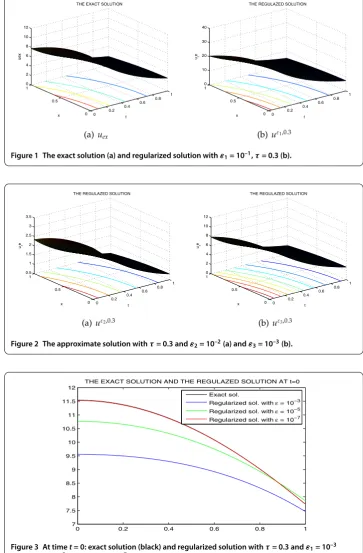
Situation: Situation focuses mainly on the regularization parameter ε. Fixτ = . and letε= –,ε= –,ε= –. We have the graphics of the exact solution and the
regularized solution with various values ofε(see Figures and ). At the initial timet= , we have the graphic in Figure .
Figure 1 The exact solution (a) and regularized solution withε1= 10–1,τ= 0.3 (b).
Figure 2 The approximate solution withτ= 0.3 andε2= 10–2(a) andε3= 10–3(b).
Figure 3 At timet= 0: exact solution (black) and regularized solution withτ= 0.3 andε1= 10–3
Table 1 The error and relative error of method in this paper withτ= 0.3 and various values ofε
ε uε,0.3(·, 0) – uex(·, 0) RE(ε, 0)
ε= 10–3 8.48702923827765 0.115626406608408
ε= 10–4 5.84620043944197 0.079648028791562
ε= 10–5 3.59734075211554 0.049009797519858
ε= 10–6 0.723559578438893 0.009857700695156
ε= 10–7 0.0550576642083171 0.000173396997915
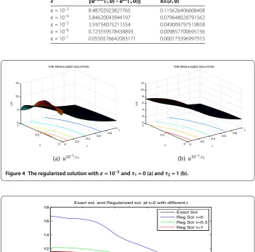
Figure 4 The regularized solution withε= 10–3andτ
1= 0 (a) andτ2= 1 (b).
Figure 5 At timet= 0: exact solution (black) and regularized solution withε= 10–3andτ= 0 (blue), τ= 0.3 (green) andτ= 1 (red).
In addition to the graphics, a table of the summary of the error estimation and relative error of the estimation is also provided (see Table ).
Remark Through Figure , Figure , Figure , and Table , it is clear that as the measur-ing errorεbecomes small, the regularized solution gets ever more close to the exact one. It is also noted that the value ofapranges from –. to . in this situation.
Situation: In this situation, the regularized parameterτis heavily focused. Fixε= –
Remark Figure and Figure agree with the theoretical result in Section : the regular-ized solution with higher value ofτis more close to the exact one. The parameterτis very useful in the case that we want to get a more accurate approximation while the measuring process cannot be better or the cost of better measuring is very expensive. In this case, with the appearance ofτ, the error can be improved without any more cost on measuring (as we can see in Figure ). It is also noted that the value ofapranges from –. to . in this situation.
Competing interests
The authors declare that they have no competing interests.
Authors’ contributions
All authors read and approved the final version of the manuscript.
Author details
1Division of Computational Mathematics and Engineering, Institute for Computational Science, Ton Duc Thang University,
Ho Chi Minh City, Vietnam.2Faculty of Mathematics and Statistics, Ton Duc Thang University, Ho Chi Minh City, Vietnam. 3Faculty of Mathematics and Computer Science, University of Science, Ho Chi Minh City, Vietnam.
Acknowledgements
The authors would like to thank Professor Dang Duc Trong and Associate Professor Nguyen Huy Tuan for the great support during their undergraduate period.
Received: 8 September 2016 Accepted: 16 January 2017
References
1. Tikhonov, AN, Arsenin, VY: Solutions of Ill-Posed Problems. V.H. Winston, Washington (1977) 2. Glasko, VB: Inverse Problems of Mathematical Physics. AIP, New York (1984)
3. Showalter, RE: The final value problem for evolution equations. J. Math. Anal. Appl.47, 563-572 (1974) 4. Showalter, RE: Quasi-reversibility of first and second order parabolic evolution equations. In: Improperly Posed
Boundary Value Problems, pp. 76-84. Pitman, London (1975)
5. Clark, GW, Oppenheimer, SF: Quasireversibility methods for non-well posed problems. Electron. J. Differ. Equ.1994, 8 (1994)
6. Fu, CL, Qian, Z, Shi, R: A modified method for a backward heat conduction problem. Appl. Math. Comput.185, 564-573 (2007)
7. Fu, CL, Xiong, XT, Qian, Z: Fourier regularization for a backward heat equation. J. Math. Anal. Appl.331, 472-480 (2007) 8. Hao, DN, Duc, NV: Stability results for the heat equation backward in time. J. Math. Anal. Appl.353, 627-641 (2009) 9. Muniz, BW: A comparison of some inverse methods for estimating the initial condition of the heat equation.
J. Comput. Appl. Math.103, 145-163 (1999)
10. Tautenhahn, U: Optimality for ill-posed problems under general source conditions. Numer. Funct. Anal. Optim.19, 377-398 (1998)
11. Abramowitz, M, Stegun, IA: Handbook of Mathematical Functions. Dover, New York (1972)
12. Trong, DD, Tuan, NH: Regularization and error estimate for the nonlinear backward heat problem using a method of integral equation. Nonlinear Anal.71, 4167-4176 (2009)
13. Trong, DD, Quan, PH, Khanh, TV, Tuan, NH: A nonlinear case of the 1-D backward heat problem: regularization and error estimate. Z. Anal. Anwend.26, 231-245 (2007)
14. Trong, DD, Tuan, NH: Regularization and error estimate for the nonlinear backward heat problem using a method of integral equation. Nonlinear Anal., Theory Methods Appl.71, 4167-4176 (2009)
15. Tuan, NH, Hoa, NV: Determination temperature of a backward heat equation with time-dependent coefficients. Math. Slovaca62, 937-948 (2012)
16. Hao, DN, Duc, NV, Lesnic, D: Regularization of parabolic equations backward in time by a non-local boundary value problem method. IMA J. Appl. Math.75, 291-315 (2010)
17. Hao, DN, Duc, NV: Regularization of backward parabolic equations in Banach spaces. J. Inverse Ill-Posed Probl.20, 745-763 (2012)
18. Cheng, W, Fu, CL: A spectral method for an axisymmetric backward heat equation. Inverse Probl. Sci. Eng.17, 1081-1093 (2009)
19. Cheng, W, Fu, CL, Qin, FJ: Regularization and error estimate for a spherically symmetric backward heat equation. J. Inverse Ill-Posed Probl.19, 369-377 (2011)
20. Denche, M, Bessila, K: A modified quasi-boundary value method for ill-posed problems. J. Math. Anal. Appl.301, 419-426 (2005)
21. Evans, LC: Partial Differential Equations. Am. Math. Soc., Providence (1998)