The importance of climatic and ecological factors for vector-borne infections: Culex pipiens and West Nile virus

(1)

U

NIVERSITY OF

T

RENTO

D

OCTORAL THESIS IN

M

ATHEMATICS

, XXIX

CYCLE

The importance of climatic and

ecological factors for vector-borne

infections:

Culex pipiens

and West

Nile virus

PhD candidate:

Giovanni Marini

Supervisors:

Prof. Andrea Pugliese Dr. Roberto Rosá

(2)

(3)

Contents

Introduction 1

1 Early warning of West Nile virus mosquito vector: climate and land use models successfully explain phenology and abundance of Culex pipiens

mosquitoes in Northwestern Italy 7

1.1 Introduction . . . 7

1.2 Methods . . . 9

1.2.1 Mosquito data . . . 10

1.2.2 Environmental predictors . . . 10

1.2.3 Temporal windows . . . 11

1.2.4 Data analysis . . . 12

1.3 Results . . . 13

1.3.1 Mosquito indices . . . 13

1.3.2 Model results . . . 14

1.4 Discussion . . . 19

1.5 Conclusions . . . 20

1.A Supporting information . . . 21

1.A.1 Aggregation of environmental data over a range of time windows: preliminary analyses . . . 21

1.A.2 Selection of the optimum 12 week time window using variation in AIC (∆AIC) . . . 24

1.A.3 Model selection tables . . . 25

2 The role of climatic and density dependent factors in shaping mosquito population dynamics: the case ofCulex pipiensin Northwestern Italy 27 2.1 Introduction . . . 27

2.2 Methods . . . 29

2.2.1 Data . . . 29

2.2.2 Modelling mosquito dynamics . . . 30

2.2.3 Model calibration . . . 31

2.3 Results and discussion . . . 32

2.A Supporting Information . . . 40

2.A.1 Materials and methods . . . 40

(4)

3.1 Introduction . . . 47

3.2 Methods . . . 49

3.2.1 Study area and mosquito data . . . 49

3.2.2 Delay analysis . . . 50

3.2.3 Environmental data . . . 50

3.2.4 Population model . . . 51

3.3 Results . . . 52

3.4 Discussion . . . 55

3.A.1 Model calibration . . . 59

3.A.2 Model output . . . 60

3.A.3 Model fit . . . 61

3.A.4 DIC and AIC analysis . . . 62

3.A.5 Estimates of the competition-dependent additional mortality . . . . 62

4 Exploring vector-borne infection ecology in multi-host communities: a case study of West Nile virus 67 4.1 Introduction . . . 67

4.2 The model . . . 68

4.2.1 Infections without horizontal transmission . . . 70

4.2.2 Horizontal transmission . . . 71

4.3 Numerical example . . . 72

4.3.1 Effect of vector and host ecology onR0 . . . 72

4.3.2 Effect of competition and shifting mosquito feeding preference on infection seasonal dynamics . . . 75

Conclusions 89

Acknowledgments 91

(5)

Introduction

More than 10% of the human deaths occurring worldwide are caused by infectious and parasitic diseases (World Health Organization, 2016). There exists a large variety of pathogens, responsible for such diseases, many of which are not directly transmitted from host to host but need a vector to be spread, such as ticks or mosquitoes. Through their bite, vectors might acquire the pathogen from infected hosts, and once infected they can transmit it to a susceptible host. These infections might affect several ani-mal species, and those that can naturally be transmitted from aniani-mals to humans are called zoonosis. Direct zoonosis, such as influenza or rabies, are directly transmitted from animals to humans, through air or bites and saliva, while for vector-borne zoonosis transmission can take place through a vector that acts as a bridge for pathogen trans-mission. About three quarters of human emerging infectious diseases are caused by zoonotic pathogens, and many of them are spread by vectors such as mosquitoes (Taylor

et al., 2001). The possibilities for emergence and spread of new zoonoses in the next future are likely to rise as world population, urbanization and human movement are constantly increasing.

Mathematical models nowadays represent very powerful tools to make investigations and predictions for biological dynamical systems, providing helpful insights that can be extremely valuable for several aims. For instance, they can assess the efficacy of a vac-cination strategy, they can help to design vector control treatments in a specific location and more generally they allow exploring what-if scenarios. As such systems evolve un-der stochastic forces, computational tools that include random influences are crucial to understand infections dynamics, including the underlying vector (if any) population fea-tures.

(6)

signs of encephalitis, meningo-encephalitis or meningitis, are often observed among el-derly people; for instance, about 220 cases were recorded in Italy between 2013 and 2016 (European Centre for Disease Prevention and Control, 2016). Several WNV epidemics have been documented in European countries in recent years (European Centre for Dis-ease Prevention and Control, 2014), and such outbreaks, as well as the quick spread of the virus throughout North America since 1999, have led to increasing health concerns (Campbellet al., 2002).

Figure 1:WNV cycle.Scheme of WNV routes of transmissions.

Mosquitoes belonging to the Cx. pipiens complex are thought to be the most efficient vectors for spreading WNV among birds, and from birds to humans and other mammals in North America (Bernard et al., 2001; Kilpatricket al., 2005) as well as in Europe (Zeller & Schuffenecker, 2004). Cx. pipiensis an indigenous species which can be found in almost every European country (Farajollahiet al., 2011). Its life cycle, similar to any other mosquito species, includes several stages, as illustrated in Figure 2. Female adults lay new eggs on water surfaces and, after hatching, larvae develop in the water and then enter a pupal stage, after which new adults will emerge. Only adult females need to have a blood meal on a host in order to to lay eggs.

Beside WNV,Cx. pipiensis also involved in the transmission of other human and ani-mal pathogens such as Usutu virus, whose first case outside Africa was recorded in Italy in 2009, St. Louis encephalitis, which caused about a hundred human cases in North America during the last decade, Rift Valley fever, Sindbis virus, avian malaria and filar-ial worms.

(7)

3

at the end of the last century; since then, Ae. albopictus rapidly spread in urban and suburban environments, occupying a habitat already exploited byCx. pipiens. It is now present in every Italian region and it is a great health concern as it is a vector for sev-eral pathogens (e.g. Zika, dengue, Chikungunya). Finally, it has been shown that Cx. pipiensmosquitoes do not bite avian hosts randomly but there are some highly preferred species, and such feeding preferences can vary during the season also depending on host availability (Kilpatricket al., 2006a; Rizzoliet al., 2015). Clearly, biting habits might strongly affect pathogens, in particular WNV, transmission.

Figure 2:Mosquito life cycle.Adults lay eggs on the water surface; the larval and pupal stages are aquatic.

In this thesis I present some mathematical models that provide insights on several as-pects of mosquito population dynamics. Specifically, I will investigate the effect of biotic and abiotic factors onCx. pipiensdynamics by using adult mosquito trapping data, gath-ered over several years in Northern Italy, to feed theoretical models.

(8)

In this thesis I will make a large use of two different kinds of model, namely statistical and mechanistic. The former are based on a hypothesized relationship between the vari-ables in an observed dataset, where the relationship seeks to best describe the data. On the other hand, in mechanistic models the nature of the relationship is specified in terms of the biological processes that are thought to have given rise to the observed data, thus the parameters in such models all have biological definitions. Throughout the thesis I will answer several ecological questions by using different statistical and computational approaches, including for instance Generalized Linear Models (GLM) and Markov chain Monte Carlo (MCMC) technique. Finally, I would like to remark that developing a useful model does not require broad mathematical skills only but also a good knowledge of all biological aspects involved in the observed data, and that interaction with biologists is essential for that.

Below I am presenting a brief description of each chapter of my thesis.

Thesis outline

The main body of my thesis is a collection of four published scientific articles, so each chapter has its own introduction, methods, results and discussion sections.

In Chapter 1 we analyze the population dynamics of Cx. pipiens in Piedmont region (Northwestern Italy) using capture data gathered in about forty different locations dur-ing years 2000-2011. Specifically, several statistical models are developed aimdur-ing to determine early warning predictors of between year variations in mosquito population dynamics. We found that climate data collected early in the year, in conjunction with local land use, can be used to provide early warning of both the timing and magnitude of mosquito outbreaks.

Chapter 2 presents a density-dependent stochastic model that describes temporal vari-ations ofCx. pipienspopulation dynamics including the effect of temperature and day-light duration on the abundance of both adults and immature stages ofCx. pipiens. The model is tailored to fit the temporal pattern of spatially averaged captures presented in Chapter 1; the results provide quantitative estimates on the effect of temperature and density-dependence onCx. pipiensabundance.

Chapter 3 presents one of the first modeling effort aiming to quantify the effect of larval interspecific competition betweenAe. albopictusandCx. pipiens. Such interaction is in-vestigated through a mechanistic model that integrate theCx. pipiensmodel presented in Chapter 2 and the Ae. albopictusmodel already present in literature (Polettiet al., 2011; Guzzettaet al., 2016a,b), using capture data of both species collected in Trentino and Veneto regions (Northeastern Italy) in 2014-2015.

(9)

5

(10)

(11)

1

Early warning of West Nile virus mosquito

vector: climate and land use models

successfully explain phenology and

abundance of

Culex pipiens

mosquitoes in

Northwestern Italy

Roberto Rosáa, Giovanni Marinia,b, Luca Bolzonia,c, Markus Netelera, Markus Metza, Luca Delucchia, Elizabeth Chadwickd, Luca Balboe, Andrea Moscae, Mario Giacobinif, Luigi Bertolottif, Annapaola Rizzolia

a: Department of Biodiversity and Molecular Ecology, Research and Innovation Centre, Fondazione Ed-mund Mach, San Michele all’Adige (TN), Italy

b: Department of Mathematics, University of Trento, Trento, Italy

c: Istituto Zooprofilattico Sperimentale della Lombardia e dell’Emilia Romagna, Parma, Italy

d: Cardiff University, School of Biosciences, The Sir Martin Evans Building, Museum Avenue, CF10 3AX Cardiff, Wales

e: Istituto per le Piante da Legno e l’Ambiente - IPLA S.p.a., Torino, Italy

f: Dipartimento di Scienze Veterinarie, Universitá degli Studi di Torino, Torino, Italy

Parasites & Vectors2014; 7: 269

1.1

Introduction

West Nile virus (WNV) is a flavivirus of emerging public health relevance in Europe (European Centre for Disease Prevention and Control, 2013). In nature it is maintained in enzootic cycles between avian reservoir hosts and mosquitoes. Humans are dead-end hosts in which infection can induce symptoms from mild flu-like fever to severe neuro-logical syndromes such as meningitis, encephalitis, and acute flaccid paralysis (Sambri

et al., 2013).

Prevention by vaccination has been possible for horses since 2003, but a human vac-cine is not yet available (Iyer & Kousoulas, 2013). Discovered originally in Uganda in 1937 (Smithburnet al., 1940), WNV is now found on every continent except Antarctica (Reisen, 2013). Several epidemics have been documented in European countries during the last 4 years (European Centre for Disease Prevention and Control, 2013), and this recent upsurge in outbreaks within endemic areas, as well as the spread of the virus throughout the New World since 1999, have led to increasing health concerns (Campbell

et al., 2002). Effective prevention and control policies are dependent on both a clearer un-derstanding of the risk factors associated with infection, and advance warning of likely outbreaks.

(12)

2013). However, implementing mosquito control measures in response to reports of hu-man cases typically is ineffectual because most huhu-mans have been infected by this time and cases appear at the end of the mosquito season, when populations are already in decline (European Centre for Disease Prevention and Control, 2013; Winters et al., 2008). Early warnings of mosquito outbreaks would provide a much needed prediction of spill-over risk (Yanget al., 2009; Cleckneret al., 2011; Deichmeister & Telang, 2011), enabling more timely control measures to be implemented, especially within WNV cir-culation areas.

Mosquitoes belonging to theCx. pipienscomplex are thought to be the most efficient vec-tors for spreading WNV among birds, and from birds to humans and other mammals in North America (Bernardet al., 2001; Kilpatricket al., 2005) as well as in Europe (Zeller & Schuffenecker, 2004). They are also involved in the transmission of other human and animal pathogens such as Usutu virus (Gaibaniet al., 2013), avian malaria and filarial worms (Farajollahiet al., 2011).

Cx. pipiensmosquitoes lay their eggs in water, and larval stages are aquatic. Aquatic habitats are therefore a prerequisite for mosquito populations, and rainfall is impor-tant in creating and maintaining suitable larval habitats (Becker et al., 2010), thus strongly affecting the abundance of adult mosquitoes (Degaetano, 2005). Temperature also strongly influences distribution, flight behaviour and dispersal, and abundance of mosquitoes (Becker et al., 2010). Specifically, temperature impacts on several aspects of the Cx. pipienslife cycle including development rates (Loetti et al., 2011; Geery & Holub, 1989), gonotrophic cycle length (Clements, 1992) and diapause duration (Spiel-man, 2001) as well as the duration of the extrinsic incubation period of the virus (Kil-patrick et al., 2008). Urban infrastructure often provides key habitats for Cx. pipiens, reflecting its affinity for stagnant water and urban areas where artificial containers of water are numerous (Deichmeister & Telang, 2011; Trawinski & Mackay, 2010). Veg-etation density is also important, due both to a positive correlation with abundance of preferred avian host species (Brownet al., 2008), and because trees and shrubs may offer resting habitats and sugar sources to adults (Gardneret al., 2013). Mosquito population density therefore reflects a complex interaction among climate, land use and vegetation coverage.

In order to develop robust statistical models to predict mosquito population dynamics, detailed data are needed describing the phenology and abundance of mosquito popula-tions, and associated environmental data at a suitable spatial and temporal resolution to act as predictor variables. Both the spatial and temporal range and resolution will determine the accuracy and range over which resulting model predictions can be made. In the Piedmont area of northern Italy, an extensive mosquito trapping programme has been in place since 1997, run by the Municipality of Casale Monferrato until 2006, and then by the Istituto per le Piante da Legno e l’Ambiente (IPLA). The area is at risk from WNV, having suitable vector and reservoir host populations, and increasing numbers of human cases of WNV in adjacent areas (Barzonet al., 2013; Monacoet al., 2010; Cal-istriet al., 2010).

Detailed environmental data are available at suitable spatial and temporal resolution across the area, thus providing an excellent system to test predictors of mosquito popu-lation dynamics. Similarities of climate and land use (Rizzoliet al., 2009) allow model predictions to be cautiously applied across northern Italy, where WNV has been circu-lating since 2008 (Calistriet al., 2010).

(13)

be-Early warning ofCx. pipiens 9

tween weekly mosquito abundance (various species) and a range of environmental data, including land use and weekly averaged climate, during the time period 10-17 days prior to measures of mosquito populations (Bisanzioet al., 2011). This approach tested for pre-dictors that immediately preceded short term variation in weekly mosquito abundance. Here we followed a different approach, aiming to determine early warning predictors of between year variation in mosquito population dynamics. We focused on Cx. pipiens

and we extended the dataset for analysis until 2011. The objective was to identify the best early warning predictors of annual variation in Cx. pipiensabundance and phe-nology, with the ultimate goal to guide entomological surveillance and thereby facilitate monitoring of WNV transmission risk.

1.2

Methods

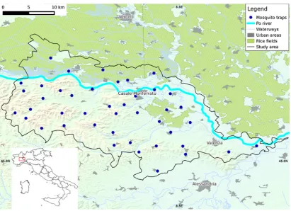
The study area encompassed 987 km2of the eastern Piedmont Region of north-western Italy (centroid: 45.07◦N, 8.39◦E) (see Figure 1.1). There are highly suitable habitats for avian hosts of WNV, and breeding sites for mosquitoes, in close conjunction to human habitation. The landscape is primarily agricultural (mixed agriculture 72%, rice fields 14%), with areas of deciduous forest on the southern hills, and riverine habitat in the north (for further details see (Bisanzioet al., 2011)). The climate is characterised by cold winters and warm summers (0.4 and 24◦C respectively), and abundant precipitation (about 600 mm/yr) primarily falling in spring and autumn (Bisanzioet al., 2011).

(14)

1.2.1 Mosquito data

Mosquitoes were collected using CO2 baited traps, operated by Municipality of Casale Monferrato and the Istituto per le Piante da Legno e l’Ambiente (IPLA) (Bisanzioet al., 2011). Trapping sites were dispersed throughout the study area, with a minimum dis-tance of 5 km between traps. Specific placement was based on coverage of all habitats deemed suitable for mosquitoes, in all participating municipalities, while enabling esti-mation of urban nuisance, and avoiding external disturbing factors (e.g. lighting, CO2 sources). Further details are provided in (Bisanzio et al., 2011). The current study in-cludes data from 2001 to 2011, collected at 44 different sites (including 28-40 sites and an average of 37 sites activated each year) (see Figure 1.1). Although most traps were run throughout, variation in activation at some sites occurred depending on the participa-tion of individual municipalities in the scheme. Alongside monitoring efforts, mosquito control strategies have been implemented in the study area since 1998 (Bisanzio et al., 2011). However, the target of all treatments wasOchlerotatus caspius, and analyses (not presented here) showed thatCx. pipiensmosquitoes were not affected by interventions. Traps were set one night every week, for a twenty-week period starting at the beginning of May and ending in mid-September, thus encompassing the main period of mosquito activity. Traps were collected the following day, and the catch counted, sexed and iden-tified. Each year since 2009, mosquitoes captured during a 6-7 night period at several sites (an average of 5 sites per year) have been pooled and tested for WNV. Until now no positive results have been found. For each trap, in every year, we (i) summed the total number of Cx. pipienscaptured during the twenty-week survey period (TOTAL), (ii) calculated the week by which 5% and 95% of the population were captured, these being designated the start (ON) and end (OFF) of the mosquito season, respectively, and (iii) calculated the number of weeks between the arrival of 5% and 95% of the trapped population, this designated as season length (SEASL). As in (Jouda et al., 2004), our definitions of ON and OFF are threshold values for population abundance, and do not necessarily reflect the cessation or initiation of diapause. Peak abundance within years was considered in preliminary analyses as a fourth measure of population dynamics, but was illdefined and unpredictable, therefore results are not presented here.

1.2.2 Environmental predictors

Environmental predictors were selected based on published evidence of their importance to mosquito populations (Degaetano, 2005; Gardneret al., 2013; Bisanzioet al., 2011; Chuang et al., 2012). All environmental data were processed in GRASS GIS (Neteler

et al., 2012), and extracted from the spatial database at the point corresponding with trap location. Cx. pipienshave a very limited dispersal (a few hundred metres (Becker, 1997)), which is within the pixel size for most spatial data (below), so data averaging over a wider area was not considered appropriate.

Climate

(15)

Early warning ofCx. pipiens 11

recorded twice daily. The original MODIS LST products were reconstructed at 250 m resolution, i.e. gap-filled to remove void pixels due to clouds (Neteler, 2010; Metzet al., 2014). For analyses, LST data were used to derive two values: (i) weekly mean LST, and (ii) a cumulative measure of temperature named here “growing degree weeks” (GDW) (see (Ruizet al., 2010)). This was derived by taking the positive difference in each week between mean LST and a threshold of 9◦C (mosquitoes fail to develop below this thresh-old, see (Loetti et al., 2011)). Weekly differences were summed cumulatively from the first week of the year, so that then-th GDW was obtained by summing thenconsecutive differences (negative differences were assigned a value of zero).

Vegetation and water indices

Normalized Difference Vegetation Index (NDVI) was obtained from the MODIS product MOD13Q1, recorded every 16 days, and the Normalized Difference Water Index (NDWI) derived from the MODIS product MOD09A1, recorded every 8 days, both at 500 m res-olution. For both the NDVI and the NDWI data, gaps were filled and outliers removed using a harmonic analysis of each time series (Roerinket al., 2000). These data were used as proxies for vegetation coverage (NDVI) (Estalloet al., 2012) and for environmen-tal water (NDWI), which includes surface water (McFeeters, 2013) as well as vegetation water content (Estalloet al., 2012).

Land use

The distance from every sampling site to the nearest urban centre (DIST_URBAN) and rice field (DIST_RICE) was calculated using the Corine Land Cover raster dataset (using the CORINE classes 111 and 112 to map the urban settlements and 213 for the rice fields (European Environment Agency, 2014) both at 100 m resolution).

1.2.3 Temporal windows

We built 22 temporal windows by grouping periods of 12 consecutive weeks, starting from the first week of the year (weeks 1-12) and ending with weeks 22-33 (approximately the end of May to mid-August). The 22 windows were divided into two groups: the first ten windows (1-12, 2-13, etc., to 10-21) were designated the “early period” and latter twelve windows (11-22, 12-23, etc., to 22-33) were designated the “late period”. The start of the mosquito season, “ON”, occurred on average during week 25, so our definition of early period predictors were those that were completed at least four weeks prior to this (i.e. ending weeks 10-21).

For each 12-week window, mean values were calculated for land surface temperature and vegetation indices (LST, NDVI and NDWI), whereas precipitation data were summed (TOT_PREC and DAY_PREC). For GDW, the cumulative value achieved by the end of the given window was used. Where these data are described in the text, the relevant temporal window is denoted in subscript, e.g. LST₁₋₁₂for mean land surface tempera-ture during weeks 1-12.

(16)

data over shorter windows (see section 1.A.1).

1.2.4 Data analysis

We investigated the association betweenCx. pipiensabundance (TOTAL) and seasonal-ity (the start of the mosquito season, ON, and season length, SEASL, as defined above), and a range of environmental predictors. All statistical analyses were performed using R version 3.0.2 (R Development Core Team, 2008). Dependent variables were transformed prior to analysis in order to normalize their distribution, following the Box-Cox method (Box & Cox, 1964). Transformations applied werex1.3for ON andx0.2for TOTAL while data for season length were normally distributed.

Preliminary analyses

Linear mixed effect models were used to ascertain, for each climatic variable, vegetation index and water index in turn, (i) which of the early period windows proved to be the best predictor of the start of the season (ON), and (ii) which of all the time windows (early and late) proved to be the best predictor of mosquito abundance (TOTAL) and season length (SEASL). In all models, trap identification number was included as a random variable. Models were ranked using the Akaike Information Criterion (AIC) (Akaike, 1974), and for each climatic variable and vegetation/water index, the time window producing the lowest AIC was selected for inclusion in subsequent full models. For NDWI the first eight time windows were not included in preliminary analyses due to the potential presence of snow cover, which can dramatically alter the reliability of satellite acquisition of this parameter (Xiao et al., 2002; Delbart et al., 2005). Terms that were not significant for any of the early or late time periods were not included in the full model. Variance Inflation Factor (VIF) (Pan & Jackson, 2008) was used to test for collinearity between all explanatory variables. Where collinearity was significant (VIF values >4, (Pan & Jackson, 2008)), the variable producing the higher AIC was excluded. This led to the exclusion of GDW and total precipitation from further analyses. Vegetation and water indices were not correlated; however, NDVI was not significant in any of preliminary models, thus it was excluded from further analyses.

Full models

(17)

the best models were ranked according to their importance (weight), i.e. the cumula-tive Akaike weight (wAIC) of the models that include that explanatory variable (Barton, 2013; Whittingham et al., 2006). This provides an idea of the frequency with which the predictor was included in the most likely models, and not directly the importance of its effect on the predicted variable. Average coefficient for each variable was calculated following modelling average procedure (Burnham & Anderson, 2002).

In order to quantify the effect size of each predictor variable, predictions were made from the best models for each significant predictor variable in turn. For predictive models, all variables but one were fixed at their average values, and predictions made across the full range of the selected variable. For example, to test the association between temperature and the start of the mosquito season (ON), in a model where temperature, precipitation and NDWI were significant predictors, precipitation and NDWI were entered into the model as constants (fixed at their average measured value), while values for tempera-ture were allowed to vary within their observed range. Models and plots were created using transformed data (for ON and TOTAL); predictions described in the text use back-transformed values to aid interpretability.

1.3

Results

1.3.1 Mosquito indices

The start of the mosquito season (ON) typically occurred during weeks 24-27 of the year (see Figure 1.2a), and the main capture period (SEASL) lasted for 56-70 days (see Figure 1.2b). The number of individuals captured (TOTAL) varied between 44 and 4648 per trap per year; more precisely, for one third of the traps the observed abundances varied between 44 and 500, for another third between 500 and 1000 and the remainder between 1000 and 4648 individuals (see Figure 1.2c).

(18)

1.3.2 Model results

Preliminary analyses

For prediction of the start of the season (ON), the optimum time windows selected for inclusion in the model were weeks 8-19, 6-17, and 10-21 for temperature (LST), pre-cipitation (DAY_PREC) and NDWI respectively (determined by comparison of AICs, see Figure 1.6). For prediction of season length (SEASL) using only early period predictors, the optimum windows for temperature and NDWI were the same as for prediction of ON (8-19; 10-21) but the optimum window for precipitation was earlier, weeks 2-13. Late pe-riod predictors were weeks 16-27 for temperature, 20-31 for precipitation and 11-22 for NDWI (see Figure 1.6). For prediction of mosquito abundance (TOTAL) using only early period predictors, the optimum windows for temperature and precipitation were weeks 10-21 and 1-12, respectively; NDWI was not significant for any time window. Additional late period predictors were weeks 21-32, 15-26 and 22-33 for temperature, precipitation and NDWI respectively (see Figure 1.6).

Full models

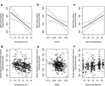
For the start of the season (ON) 32 full models were produced and a single best model was selected, explaining 26% (R2₌0.258, Akaike weight = 0.96) of the variance; remaining models had∆AIC>4 and were disregarded (see section 1.A.3). Model outputs (see Table 1.1) are therefore based on a single model, rather than averages from multiple models as elsewhere. Within the measured range of environmental data, temperature had the greatest effect on the start of the season. Higher spring temperatures were associated with an earlier start to the season, such that an increase of 5◦C in LST8−19 (from 11 to

16◦_{C) predicts the start of the season some 14 days earlier (a shift in the average ON}

from day 187 to 173) (see Figure 1.3a). Increasing NDWI also predicts an earlier start to the season, such that a shift in NDWI10−21from -0.1 to +0.06 led to a start of the season

10 days earlier (see Figure 1.3b), while more days of precipitation delayed the start of the season such that an increase in DAY_PREC6−17from 14 to 37 days of precipitation

during the 12 week period led to a delay in the start of the season of 10 days (see Figure 1.3c). All terms selected in the best models (LST8−19, NDWI10−21and DAY_PREC6−17)

were highly important with a predictor weight equal to or very close to 1 (see Table 1.1). Neither distance to urban area or rice fields were significant predictors.

When considering only the early period, two models, out of 32 models produced, were se-lected to predict season length, explaining between 13 and 14% (R2₌0.135,R2₌0.141) of the variance, and differed in their inclusion/exclusion of temperature (Akaike weights were 0.21 and 0.77). From model averaging, the early period variables associated with earlier start of the season (ON, above) also predict increased season length, so higher NDWI and temperature predict a longer season (although note that following averaging procedures temperature is significant only at a 92% threshold, with p₌0.079), and more days of precipitation predict a shorter season. Again, distance to urban areas and rice fields were not significant predictors, for either of the two best models. For early period predictors only, an increase in NDWI10−21from -0.1 to +0.06 predicts an increase of 14

days in season length (from 56 to 70 days), while an increase in days of precipitation from 7 to 30 days during the 12 week period (DAY_PREC2−13) predicts an eleven day

(19)

72 days).

Figure 1.3: Association between the start of the mosquito season and environmental variables. Panels a-c show model predictions; panels d-f show partial residuals. The first col-umn (a,d) shows the association between the start of the season and temperature (LST8−19), the second (b,e) shows the association with NDWI10−21and the third (c,f) shows the association with precipitation (DAY_PREC6−17). Note that all plots show transformed data on theyaxis (i.e.x1.3); back transformed values are presented in the text to assist interpretation.

Variable

Weight

Coeff.

Std. error

z-value

Pr(

> |

z

|

)

Intercept

1014.19

96.54

10.51

<

0.001

LST

8−19

1

-17.3

5.6

-3.09

0.002

NDWI

10−21

1

-369.07

155.43

-2.37

0.018

DAY_PREC

6−17

0.99

2.76

0.88

3.12

0.002

Table 1.1:Predicting the start of the mosquito season (ON). The weight and significance of terms remaining in the best selected model.

(20)

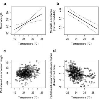
Figure 1.4:Association between season length and days of precipitation.Panels a-b show model predictions; panels c-d show partial residuals. The first column (a,c) shows the association with days of precipitation during the early period (DAY_PREC2−13) while the second column (b,d) shows the association with precipitation in the late period (DAY_PREC20−31).

during the late period (DAY_PREC20−31) has the opposite effect of precipitation during

the early period (DAY_ PREC2−13) (see Figure 1.4b). More days of precipitation during

the late period predict a longer season, such that an increase from 12 to 39 days of precip-itation (DAY_PREC20−31) predicts a seven day increase in season length, whereas in the

early period only model, more days of precipitation delay the season start and so shorten season length (as described above). The association with late period precipitation is stronger than that of early period precipitation, so that when both terms are included in the same model, early period precipitation becomes non-significant with a predictor weight of only 0.4, as compared to a high significance of p₌0.004 and a weight of 0.79 for late period precipitation (see Table 1.2). Late period temperatures (LST₁₆₋₂₇) have a marked impact on season length such that a shift of 6◦C (from 19 to 25◦C) predicts a lengthening of the season by 22 days (see Figure 1.5a). As for precipitation, the addition of late period temperature renders early period temperature non-significant, with pre-dictor weight of only 0.53, as compared to late period temperature which is both highly significant (p₌0.003) and has a high predictor weight (0.98) (Table 1.2). The most im-portant model term in terms of predictor weight was, however, NDWI measured during the early period (NDWI10−21), which is positively associated with season length, and

(21)

length of 14 or 17 days (the greater increase being predicted by the early+late models).

Model Variable Weight Coeff. Std. error z-value Pr(> |z|) Early Intercept 59.57 15.42 3.86 <0.001

NDWI10₋21 1 85.23 31.52 2.7 0.007

DAY_PREC2−13 0.99 -0.5 0.14 3.65 <0.001

LST8−19 0.78 1.5 0.85 1.76 0.079

Early+Late Intercept -19.11 28.45 0.67 0.501

NDWI10₋21 1 104.26 31.36 3.32 0.001

LST16₋27 0.98 3.78 1.26 2.98 0.003

DAY_PREC20−31 0.79 0.29 0.1 2.88 0.004

LST8−19 0.53 0.1 1.11 0.09 0.926

DAY_PREC2−13 0.4 -0.28 0.16 1.73 0.083

Table 1.2: Predicting season length (SEASL). The average weight and significance of vari-ables remaining in the two best ’Early predictors only’ and six best ’Early + Late predictors’ models. Note that terms in italics are significant in some of the selected best models but not in others, and that overall, weighted model averaging procedures suggest that they are not signifi-cant.

Of the 16 full models produced, two were selected to predict mosquito abundance (TO-TAL) from early period predictors, explaining between 46 and 49% of the variance (R2=

0.464, R2₌0.488) with Akaike weights of 0.12 and 0.79 respectively. Abundance was best predicted by early period models including days of precipitation at the start of the year (DAY_PREC1−12), and distance to rice fields. An increase in precipitation predicts

an increase in abundance (e.g. an increase from 7 to 30 days rain predicts an increase from approximately 400 to 1000 mosquitoes per trap). Traps closer to rice fields cap-tured more mosquitoes than those 13 km away (average 680 mosquitoes per trap year, compared to 560). The very different prediction weights of the two terms selected in the early period models (Table 1.3), however, indicate that while days of precipitation play an important role, distance to rice fields has a very limited effect on early period model predictions. Incorporation of additional late period predictors did not greatly im-prove the model fit; again, two models were selected, out of 128 models produced, and explained 52% of the variance (R2₌0.523,R2₌0.524) with Akaike weights of 0.35 and 0.49 respectively. Days of precipitation at the start of the year (DAY_PREC1−12)

re-mained a highly significant predictor, and predicted a similar effect (an increase from 7 to 30 days of rain predicts an increase in total abundance from 420 to 860 mosquitoes per trap year). Distance to rice fields was not a significant predictor in early+late period models, while average temperature during the late period (LST21−32) exerted a

signifi-cant negative effect on predictions, such that an increase in temperature from 21 to 30◦_C

led to a marked decrease in abundance from approximately 1150 to only 150 mosquitoes per trap year (Figure 1.5b). The days of precipitation measured during the early period (DAY_PREC₁₋₁₂) is the most important term predicting TOTAL in both groups of mod-els (early only, early+late) while temperature has a strong impact on model prediction for the early+late model only (Table 1.3). Late period NDWI (NDWI22−33) was selected

(22)

Model Variable Weight Coeff. Std. error z-value Pr(> |z|) Early Intercept 1.27 8.4e-03 152.83 <0.001

DAY_PREC1−12 1 2.8e-02 3.2e-03 8.75 <0.001 DIST_RICE 0.13 -7.8e-05 1.6e-05 4.78 <0.001 Early+Late Intercept 6.96 0.53 12.97 <0.001 LST21−32 1 -0.15 0.021 7.24 <0.001 DAY_PREC1−12 1 1.7e-02 3.1e-03 5.04 <0.001

NDWI22₋33 0.6 -0.886 1.150 0.77 0.441

Table 1.3: Predicting mosquito abundance (TOTAL). The average weight and significance of variables remaining in the two best ’Early predictors only’ and two best ’Early + Late predic-tors’ models. Note that terms in italics are significant in some of the selected best models but not in others, and that overall, weighted model averaging procedures suggest that they are not significant.

(23)

1.4

Discussion

The transmission of WNV is strongly linked to the abundance of the Culex mosquito vector (Colbornet al., 2013; Kilpatrick & Pape, 2013), and many studies have focused on describing and quantifying habitat associations and spatio-temporal distributions of the vector species to guide implementation of effective control strategies (Winterset al., 2008; Diuk-Wasseret al., 2006). In particular, early predictions of both the timing and intensity of future mosquito abundance will help to enable decision makers to apply ef-fective prevention and control plans (Yanget al., 2009).

The current study aimed to identify early warning predictors ofCx. pipiensabundance and phenology, with the ultimate goal of improving entomological surveillance and fo-cussing interventions to enable early detection of virus circulation in mosquitoes. To achieve this, we modelled the association between annual measures of mosquito abun-dance and phenology (start of the season and season length) and a set of environmental predictors.

Environmental predictors were selected based on published evidence of their importance to mosquito populations, and were averaged across twelve week periods in order to test the effect of variation at a seasonal scale, rather than focusing on daily or weekly fluctu-ations (e.g. (Bisanzioet al., 2011)).

Our results indicate that warm temperatures during the early period (prior to the main mosquito season) lead to an earlier start, and extend the duration of the mosquito season (SEASL), but are not associated with a significant increase in abundance. This is likely to result from the acceleration of mosquito development rates driven by higher tempera-tures (Loettiet al., 2011). Higher temperatures during the late period (encompassing the main period of mosquito host seeking activity) are similarly associated with increased season length, but also with a decrease in total abundance. This latter result is opposite to the one found by Bisanzio et al.(2011) but is coherent with the observed captures: for instance 2003 was the hottest summer during the current study, and also the year with the least captures. This is also consistent with results obtained from laboratory experiments where adult survival and longevity ofCx. pipienswere negatively affected by high temperatures (Ciotaet al., 2014). In addition, when high temperatures during summer are associated with low precipitation, as was the case in 2003, the combined effects of very hot and dry conditions are likely to cause rapid drying of aquatic breeding sites, with a consequent negative impact on mosquito populations. Recent observations in north-eastern Italy corroborate the negative impact of high summer temperatures, revealing a significant decline in populations when temperatures approached the maxi-mum tolerance forCx. pipiensover a prolonged period (Mulattiet al., 2014).

Early period precipitation postponed and shortened the activity of host-seeking mosquitoes, but at the same time was associated with greater abundance. Conversely, precipitation during the late period was associated with an extension of the season. An association between increased abundance and early period precipitation is probably associated with the increase in formation and persistence of mosquito breeding sites while more days of precipitation during the late period would prolong the existence of breeding pools, thus sustaining mosquito populations later in the year (Degaetano, 2005).

(24)

Good levels of moisture, especially in the soil, are a fundamental requirement for the formation and persistence of mosquito breeding sites (Estalloet al., 2012).

Although the two physical distances (to rice fields, and to urban areas) do not seem to be very important forCx. pipiensin the current study, the negative association between abundance and distance from rice fields suggests that this land use provides important habitat in north-western Italy. This result was confirmed by larval collection ofCx. pip-iens in rice-fields. Distances to urban areas were never selected in any of our models, suggesting that in this region of Italy urban settlements are not an important breeding habitat for Cx. pipiens, although it is possible that habitat type causes a bias in trap at-tractiveness. This is different to a number of other studies, carried out in North America and Europe, where it has been shown thatCx. pipiensprefers urban settlements (Deich-meister & Telang, 2011; Trawinski & Mackay, 2010; Becker, 1997). These preferences in North America may reflect differences in the ecology ofCx. pipiensin the Old, versus the New World, or may reflect differences in the biogeography of the two regions. Alter-natively, such differences may reflect the presence of different forms of the species. Form

pipiensprefers a more rural habitat, whilemolestusis more urban (Osórioet al., 2014). The form present in the eastern Piedmont area has not been definitively identified, but the relatively infrequent bites to humans (pers. obs) makespipiens(which are predom-inantly bird-feeding) the more likely. Although Bisanzio et al. (2011) present spatial analyses (based on the same area as the current study) in which the highest abundances ofCx. pipienswere close to urban areas, the term was not significant in their final model. The equivocal nature of the results suggested by Bisanzio et al.(2011), and the lack of support for urban preference in the current study, using a longer timeseries, supports a view that urban areas are of limited importance toCx. pipiensin north western Italy.

1.5

Conclusions

(25)

1.A

Supporting information

1.A.1 Aggregation of environmental data over a range of time windows:

preliminary analyses

In order to select an appropriate period of time for aggregation of environmental data, we ran preliminary analyses comparing single model predictions of mosquito indices (ON, SEASL and TOTAL). Explanatory variables were the environmental predictors (DAY_PREC, LST or NDWI), and data for each environmental predictor were summed (DAY_PREC) or averaged (LST and NDWI) within each temporal window, using a range of aggregation periods: 1, 2, 4, 8, 12 weeks.

Comparisons were therefore made between:

• 1 week aggregation, producing 33 temporal windows from week 1 until week 33;

• 2 week aggregation, producing 32 temporal windows from weeks 1-2 until weeks 32-33;

• 12 week aggregation, producing 22 temporal windows from weeks 1-12 until weeks 22-33.

To make comparisons between models we looked at:

• The percentage of models with significant coefficients (Table 1.4).

• Consistency - estimated by how many times the coefficients from models using two consecutive temporal windows changed their sign (Table 1.5).

• Minimum and Mean values of model AIC (Tables 1.6 and 1.7).

(26)

Aggregation period (weeks) 1 2 4 8 12 ON DAY_PREC 0.95 0.75 0.78 0.93 1.00 LST 0.67 0.70 0.94 1.00 1.00 NDWI 0.38 0.42 0.40 0.83 1.00 SEASL DAY_PREC 0.70 0.63 0.77 0.77 0.86 LST 0.61 0.59 0.77 0.88 1.00 NDWI 0.20 0.29 0.18 0.28 0.29 TOTAL DAY_PREC 0.58 0.63 0.63 0.81 0.95 LST 0.70 0.75 0.73 0.65 0.64 NDWI 0.20 0.25 0.27 0.28 0.07 All models 0.55 0.56 0.61 0.71 0.76

Table 1.4: Significance of coefficients (%).

Aggregation period (weeks) 1 2 4 8 12 ON DAY_PREC 7 5 3 0 0

LST 3 3 0 0 0

NDWI 0 2 0 0 0

SEASL DAY_PREC 12 8 4 2 1

LST 9 7 2 0 0

NDWI 4 4 2 2 2

TOTAL DAY_PREC 16 6 4 0 0

LST 6 6 4 2 2

NDWI 6 2 1 1 1

All models 63 43 20 7 6

Table 1.5: Number of changes of coefficient sign.

Aggregation period (weeks)

1 2 4 8 12

ON DAY_PREC 4860.36 4729.09 4733.10 4726.25 4733.78 LST 4862.16 4744.36 4750.51 4748.47 4730.55 NDWI 4438.35 4781.76 4786.31 4796.04 4801.20 SEASL DAY_PREC 4865.77 4731.22 4734.31 4731.77 4724.15 LST 4866.80 4749.80 4751.50 4751.80 4719.20 NDWI 4438.79 4779.01 4783.42 4792.01 4780.82 TOTAL DAY_PREC 763.36 618.80 634.67 637.49 651.26 LST 764.49 656.40 624.28 610.83 623.34 NDWI 688.14 700.33 700.12 695.43 702.88 All models 3394.25 3387.86 3388.69 3387.79 3385.24

(27)

Aggregation period (weeks)

1 2 4 8 12

ON DAY_PREC 4912.25 4786.94 4778.19 4759.43 4759.40 LST 4909.12 4785.25 4781.99 4771.03 4767.06 NDWI 4777.65 4793.08 4797.79 4799.93 4801.62 SEASL DAY_PREC 4912.70 4788.84 4786.97 4780.72 4774.71 LST 4927.64 4807.04 4811.70 4812.60 4797.89 NDWI 4777.19 4793.76 4798.80 4801.72 4792.06 TOTAL DAY_PREC 809.38 699.33 703.82 694.19 697.41 LST 804.86 691.83 692.36 678.22 682.99 NDWI 805.29 712.60 716.84 698.18 707.00 All models 3515.12 3428.74 3429.83 3421.78 3420.02

(28)

1.A.2 Selection of the optimum 12 week time window using variation

in AIC (

∆

AIC)

The time window producing the lowest AIC was selected for inclusion in full models.

(29)

1.A.3 Model selection tables

Models AIC ∆AIC wAIC R2

ON∼LST8−19+ DAY_PREC6−17+ NDWI10−21 4687.93 0.00 0.962207 0.258 ON∼DIST_URBAN + LST8−19+ DAY_PREC6−17+ NDWI10−21 4695.29 7.36 0.024327 0.266 ON∼LST8−19+ NDWI10−21 4697.15 9.22 9.59E-03 0.240 ON∼DAY_PREC6−17+ NDWI10−21 4700.45 12.52 1.84E-03 0.241 ON∼DIST_RICE + LST8−19+ DAY_PREC6−17+ NDWI10−21 4701.11 13.17 1.33E-03 0.258 ON∼LST8−19+ DAY_PREC6−17 4703.46 15.52 4.10E-04 0.247 ON∼DIST_URBAN + DAY_PREC6−17+ NDWI10−21 4706.06 18.12 1.12E-04 0.252 ON∼DIST_URBAN + LST8−19+ NDWI10−21 4706.28 18.35 9.99E-05 0.245 ON∼DIST_RICE + LST8−19+ NDWI10−21 4708.90 20.97 2.69E-05 0.243 ON∼DIST_URBAN + LST8−19+ DAY_PREC6−17 4710.08 22.14 1.49E-05 0.257

Table 1.8: The ten “best” full models predicting start of the mosquito season (ON) - those with lowest AIC values obtained from model selection. For each model we report AIC, the difference in AIC with respect to the best model (∆AIC), the Akaike weight (wAIC) andR2.

SEASL∼LST8−19+ DAY_PREC2−13+ NDWI10−21 3380.28 0.00 0.767278 0.141 SEASL∼DAY_PREC2−13+ NDWI10−21 3382.85 2.57 0.212613 0.135 SEASL∼LST8−19+ NDWI10−21 3388.97 8.69 9.95E-03 0.114 SEASL∼DIST_URBAN + LST8−19+ DAY_PREC2−13+ NDWI10−21 3389.89 9.61 6.28E-03 0.153 SEASL∼DIST_URBAN + DAY_PREC2−13+ NDWI10−21 3391.68 11.39 2.57E-03 0.148 SEASL∼LST8−19+ DAY_PREC2−13 3394.00 13.72 8.05E-04 0.127 SEASL∼DIST_RICE + LST8−19+ DAY_PREC2−13+ NDWI10−21 3396.14 15.86 2.76E-04 0.143 SEASL∼DAY_PREC2−13 3398.28 17.99 9.49E-05 0.116 SEASL∼DIST_RICE + DAY_PREC2−13+ NDWI10−21 3399.48 19.20 5.2E-05 0.135 SEASL∼DIST_URBAN + LST8−19+ NDWI10−21 3400.02 19.73 3.98E-05 0.123

(30)

Models AIC ∆AIC wAIC R2 SEASL∼NDWI10−21+ LST16−27+ DAY_PREC20.31 3374.32 0.00 0.283167 0.156 SEASL∼LST8.19 + NDWI10−21+ LST16−27+ DAY_PREC20.31 3374.41 0.09 0.27071 0.156 SEASL∼LST8.19 + DAY_PREC2−13+ NDWI10−21+ LST16−27+ DAY_PREC20.31 3376.08 1.76 0.117533 0.16 SEASL∼DAY_PREC2−13+ NDWI10−21+ LST16−27+ DAY_PREC20.31 3376.08 1.76 0.117364 0.16 SEASL∼LST8.19 + DAY_PREC2−13+ NDWI10−21+ LST16−27 3376.58 2.26 0.091288 0.15 SEASL∼DAY_PREC2−13+ NDWI10−21+ LST16−27 3377.55 3.23 0.056259 0.147 SEASL∼LST8.19 + NDWI10−21+ LST16−27 3378.36 4.04 0.03753 0.138 SEASL∼LST8.19 + DAY_PREC2−13+ NDWI10−21 3380.28 5.96 0.014372 0.141 SEASL∼DAY_PREC2−13+ NDWI10−21 3382.85 8.53 3.98E-03 0.135 SEASL∼NDWI10−21+ LST16−27 3383.76 9.44 2.52E-03 0.125

Table 1.10: of the ten“best” full models predicting season length (SEASL) using early and late period data - those with lowest AIC values obtained from model selection. For each model we re-port AIC, the difference in AIC with respect to the best model (∆AIC), the Akaike weight (wAIC) andR2.

TOTAL_∼DAY_PREC1−12 634.19 0.00 0.79395 0.464 TOTAL∼DIST_RICE + DAY_PREC1−12 637.92 3.73 0.12304 0.488 TOTAL∼LST10−21+ DAY_PREC1−12 638.90 4.71 0.075289 0.467 TOTAL_∼DIST_RICE + LST₁₀₋₂₁+ DAY_PREC₁₋₁₂ 644.04 9.85 5.76E-03 0.489 TOTAL_∼DIST_URBAN + DAY_PREC₁₋₁₂ 647.14 12.95 1.22E-03 0.473 TOTAL_∼DIST_URBAN + DIST_RICE + DAY_PREC1−12 648.49 14.30 6.22E-04 0.501 TOTAL_∼DIST_URBAN + LST10−21+ DAY_PREC1−12 652.21 18.03 9.67E-05 0.476 TOTAL_∼DIST_URBAN + DIST_RICE + LST10−21+ DAY_PREC1−12 655.10 20.92 2.28E-05 0.501

TOTAL∼1 692.45 58.27 1.77E-13 0.365

TOTAL∼LST10−21 693.21 59.03 1.21E-13 0.375

Table 1.11: The ten “best” full models predicting mosquito abundance (TOTAL) using early period data only - those with lowest AIC values obtained from model selection. For each model we report AIC, the difference in AIC with respect to the best model (∆AIC), the Akaike weight (wAIC) and R2.

TOTAL_∼DAY_PREC1₋12+ LST21₋32+ NDWI22₋33 592.74 0.00 0.494334 0.524 TOTAL∼DAY_PREC1−12+ LST21−32 593.42 0.68 0.351739 0.523 TOTAL_∼DIST_RICE + DAY_PREC1−12+ LST21−32+ NDWI22−33 597.94 5.20 0.036789 0.543 TOTAL_∼LST10₋21+ DAY_PREC1₋12+ LST21₋32+ NDWI22₋33 598.29 5.55 0.030896 0.526 TOTAL∼DAY_PREC1−12+ LST21−32+ DAY_PREC15−26+ NDWI22−33 598.88 6.14 0.022952 0.530 TOTAL_∼LST10−21+ DAY_PREC1−12+ LST21−32 599.18 6.44 0.019778 0.525 TOTAL_∼DAY_PREC1₋12+ LST21₋32+ DAY_PREC15₋26 599.46 6.72 0.017162 0.529 TOTAL∼DIST_RICE + DAY_PREC1−12+ LST21−32 602.01 9.27 4.80E-03 0.539 TOTAL_∼DIST_URBAN + DAY_PREC1−12+ LST21−32+ NDWI22−33 602.10 9.36 4.58E-03 0.537 TOTAL_∼DIST_URBAN + DAY_PREC1₋12+ LST21₋32 602.48 9.73 3.80E-03 0.536

(31)

2

The role of climatic and density dependent

factors in shaping mosquito population

dynamics: the case of

Culex pipiens

in

Northwestern Italy

Giovanni Marinia,b, Piero Polettic,d, Mario Giacobinie, Andrea Puglieseb, Stefano Merlerc, Roberto Rosáa

a: Department of Biodiversity and Molecular Ecology, Research and Innovation Centre, Fondazione Ed-mund Mach, San Michele all’Adige (TN), Italy

b: Department of Mathematics, University of Trento, Trento, Italy c: Bruno Kessler Foundation, Trento, Italy

d: Dondena Centre for Research on Social Dynamics and Public Policy, Department of Policy Analysis and Public Management, Universitá Commerciale L. Bocconi, Milan, Italy

e: Dipartimento di Scienze Veterinarie, Universitá degli Studi di Torino, Torino, Italy

PLoS ONE2016; 11(4): e0154018

2.1

Introduction

Zoonotic pathogens are believed to cause about three quarters of human emerging infec-tious diseases, many of which (22%) are spread by vectors such as mosquitoes (Taylor

et al., 2001). One of the most recent emerging mosquito-borne diseases in the West-ern Hemisphere is West Nile Virus (WNV), a flavivirus first isolated in Uganda in 1937 (Smithburnet al., 1940). It is maintained in a bird-mosquito transmission cycle primar-ily involving Culexspecies mosquitoes of which the Cx. pipiens complex is thought to be one of the most important in Europe (Zeller & Schuffenecker, 2004). In recent years, WNV has been circulating in many European countries, including Italy, causing hun-dreds of human cases (European Centre for Disease Prevention and Control, 2014). Cx. pipiensis also involved in the transmission of other human and animal pathogens such as Usutu virus (Gaibani et al., 2013), whose first case outside Africa was recorded in Italy in 2009 (Pecorariet al., 2009), St. Louis encephalitis (Reisenet al., 2008), which caused about a hundred human cases in North America during the last decade (Ar-boNET, 2014), Rift Valley fever (Turell et al., 2014), Sindbis virus (Lundstrom et al., 2001), avian malaria and filarial worms (Farajollahiet al., 2011).

The transmission of mosquito-borne diseases is largely driven by the abundance of the vector (Colborn et al., 2013; Kilpatrick & Pape, 2013). Thus, rigorous surveillance of mosquito density and control programs based on its reduction represent key components of disease containment and prevention. Therefore, in order to design appropriate control strategies it is crucial to understand the population dynamics of existing vector popula-tions and evaluate how it depends on environmental factors.

(32)

mosquitoes has been implemented, since 1997, by the Municipality of Casale Monfer-rato and the Istituto per le Piante da Legno e l’Ambiente (IPLA). The area is at risk for WNV, because of the presence of suitable vector and reservoir host populations, and the increasing numbers of human cases of WNV in adjacent areas (Calistriet al., 2010; Monacoet al., 2010). Previous studies ((Bisanzioet al., 2011) and Chapter 1) analyzed spatio-temporal variations of mosquito species collected in the area, detecting a very high heterogeneity in the temporal pattern of mosquito population dynamics both inter-and intra-annually. In particular, looking atCx. pipienspopulation dynamics from 2001 to 2011, we detected a huge variation in total yearly mosquito abundance among differ-ent traps, ranging from 40 to more than 4000 individuals captured per year (see Chapter 1). Also the timing of mosquito seasonal dynamics varied significantly among traps and years. Specifically, for around 90% of the observations the start of mosquito season var-ied from the beginning of June to mid-July, while the length of mosquito season varvar-ied from 45 to 90 days (see Section 1.3).

The main goal of our work is to describe and interpret in a robust theoretical frame-work the high heterogeneity observed among different seasons forCx. pipiens popula-tion dynamics in Northwestern Italy, by explicitly taking into account some important eco-climatic and biological factors.

In Chapter 1 we found that precipitation and temperatures during the early period of the year (spring and early summer) might remarkably influenceCx. pipienspopulation dynamics. In particular, warm temperatures early in the year were associated with an earlier start of the mosquito season and increased season length, while early precipita-tion delayed the start, and shortened the length of the mosquito season, but increased total abundance. Indeed, temperature is well known to affect several aspects ofCx. pip-ienslife cycle including development and survival rates (Ciotaet al., 2014; Loettiet al., 2011).

Density-dependence in mosquito population growth is another important factor in regu-latingCx. pipienspopulation dynamics (Mulattiet al., 2014). In fact, it has been found that inclusion of density-dependence, in combination with key environmental factors, significantly improves model prediction ofCx. pipienspopulation expansion in Northern Italy (Mulattiet al., 2014). By using a statistical model, the authors found that the most significant environmental drivers ofCx. pipienspopulation dynamics were the daylight duration and temperature conditions in the 15 day period prior to sampling while pre-cipitation and humidity had only a minor influence onCx. pipiensgrowth rates.

Diapause is a common mechanism adopted by mosquitoes to survive through winter. While other mosquitoes, for instance Aedes albopictus, overwinter through diapausing eggs (Denlinger & Armbruster, 2014), in the case ofCx. pipiens, only adult females un-dergo diapause halting blood feeding and therefore host-seeking behavior (Denlinger & Armbruster, 2014). More specifically, immature stages develop into diapausing adults according to the photoperiod they are exposed to (Spielman & Wong, 1973).

(33)

Ya-Eco-climatic drivers ofCx. pipiensdynamics 29

mana & Eltahir, 2013; Cailly et al., 2012)) and Ae. albopictus (e.g. (Ericksonet al., 2010; Polettiet al., 2011; Tranet al., 2013)) while, to the best of our knowledge, fewer attempts have been carried out for modelling Cx. species population dynamics (Gong

et al., 2011; Loncaric & Hackenberger, 2013; Morin & Comrie, 2010; Paweleket al., 2014). Mathematical models represent a powerful tool to investigate the role played by different climatic factors on vector population dynamics and to evaluate the effec-tiveness of alternative mosquito control strategies, as suggested by recent works onCx. quinquefasciatus(Morin & Comrie, 2010),Anophelesspecies (Caillyet al., 2012) andAe. albopictus(Tranet al., 2013). We follow a stochastic approach as deterministic models ignore the contribution of demographic stochasticity which is especially relevant when the vector population is low, for instance at the beginning and at the end of mosquito activity season. The proposed model explicitly accounts for the temporal variation of all immature stages, i.e. eggs, four larval instars and the pupal stage; it is assumed that the lengths of all mosquito life stages depend on temperature and that developmental rates of larval stages are density-dependent; finally, a diapausing mechanism is included in response to the photoperiod.

The effect of precipitation on survival and development of mosquito life stages is not explicitly accounted for, as, to the best of our knowledge, no reliable data onCx. pipiens

are present in literature for modeling and calibrating such mechanism. In the Results Section, we discuss correlation of density dependence with precipitation, which could in-directly enter the model in this way.

Finally, extensive model simulations have been carried out in order to better understand the role played by different eco-climatic factors in shaping the seasonal specific vector dynamics and to forecast, under various illustrative scenarios, likely changes inCx. pip-iensseasonal dynamics if temperature or density-dependent inputs would change.

2.2

Methods

2.2.1 Data

(34)

the area and in the human population size.

The biotype present in the eastern Piedmont area has not been definitively identified. However, given the relatively infrequent bites to humans in the considered area, in Chapter 1 we suggested Cx. pipiens pipiens which is predominantly birdfeeding -as the more likely biotype. It is possible that human exposure to mosquito bites may be lower in more agricultural areas. However, a recent study conducted in a region of Northern Italy showed thatCx. pipiensprefer to take blood meals from avian hosts both in rural and urban areas (Rizzoli et al., 2015). For a more detailed description of the study area and the trapping conditions, see (Bisanzioet al., 2011) and Section 1.2.

2.2.2 Modelling mosquito dynamics

The model for the dynamics of the abundance of the vector in seven life stages of Cx. pipiens, namely eggs (E), 4 larval instars (L1,L2,L3,L4), pupae (P) and non-diapausing

female adults (A), is based on the following system of equations:

M=                                 

E0 ₌ nE

dAA−

¡

µE+τE¢E

L0

1 = τEE−

³

τL1+µL1

³

1₊L1+L2+L3+L4 K

´´ L1

L0

2 = τL1L1−

³

τL2+µL2

³

1₊L1+L2+L3+L4 K

´´ L₂

L0

3 = τL2L2−

³

τL3+µL3

³

1₊L1+L2+L3+L4 K

´´ L₃

L0₄ = τL3L3−

³

τL4+µL4

³

1+L1+L2+L3+L4 K

´´ L4

P0 ₌ τL4L4−

¡

τP+µP¢P

A0 = 1₂τP(1−p)P−βµAA−χCαA

C0 ₌ χCαA

where_τE,τL1,τL2,τL3,τL4,τP are the temperature dependent developmental rates

driv-ing the transitions of vectors across the different life stages considered;µE,µL1,µL2,µL3,

µL4,µP, µA are the temperature dependent death rates associated with the different

stages;nEis the number of eggs laid in one oviposition;dAis the length of the gonotrophic

cycle;K is the density-dependent scaling factor driving the carrying capacity for the lar-val stages; pis the probability (depending on daylight duration) that a fully developed pupa becomes a diapausing adult; β gauges the possible increase in adult mortality rate due to wild conditions with respect to lab conditions; α is the capture rate; χC is

a function of the time defined equal to 1 when the trap is open and 0 otherwise;C rep-resents the cumulative number of captured female adult mosquitoes. Since only female adult mosquitoes are explicitly considered in the model, the term 1₂ in the equation for the adults accounts for the sex ratio (Vinogradova, 2011). Note, moreover, that dia-pausing females do not take blood meals before overwintering (Denlinger & Armbruster, 2014) and they cannot be captured with the considered traps. For this reason, only non-diapausing female adults are considered in the model.

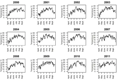
Daily mean temperature and precipitation records for the period and study area con-sidered were obtained from ARPA Piedmont (Arpa Piemonte, 2014). Daylight durations for the centroid of the study region during the considered period were obtained from the US Naval Observatory (United States Naval Meteorology and Oceanography Command, 2013).

(35)

Eco-climatic drivers ofCx. pipiensdynamics 31

developmental stages, and whose transition probabilities are built according to binomial distributions whose means are obtained from the rate in system M. Details are speci-fied in Section 2.A. The seasonal dynamics of the mosquito population is simulated for 12 years, from April 1 (corresponding to approximately one month before the first cap-ture session) to October 1. Since, to the best of our knowledge, no data are available on the overwintering ofCx. pipiens, we simulate each yearyseparately by initializing the system with A0(y)>0 non-diapausing adults.

2.2.3 Model calibration

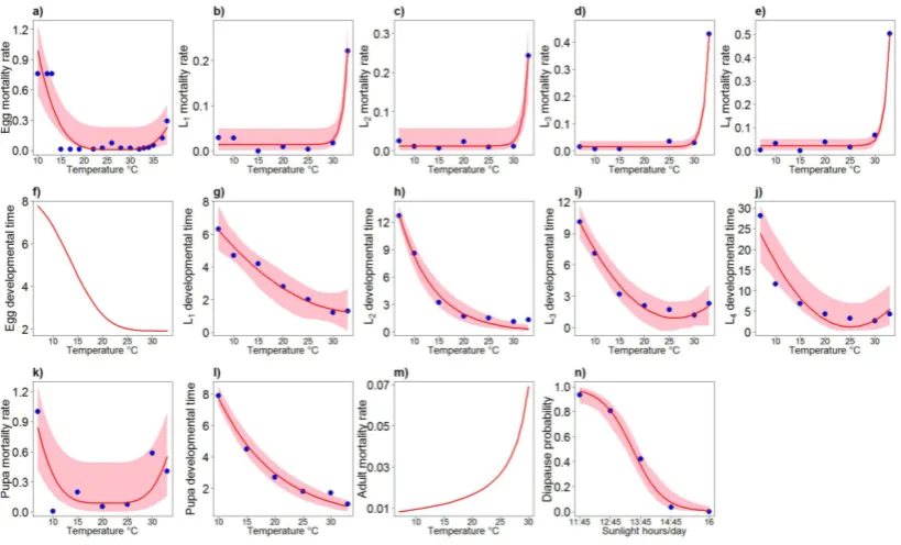
Mortality and developmental rates across different vector life stages have been mod-eled as a function of temperature following the approach already proposed in (Poletti

et al., 2011) on the basis of data collected in (Loettiet al., 2011; Eirayah & Abugroun, 1983). Specifically, we modeled the developmental period and the mortality rate as-sociated with different vector stages at each temperature by fitting a suitable set of functions of the temperature T - comprising exponential and parabolic functions - to durations and rates measured at different specific temperatures through laboratory ex-periments (Loettiet al., 2011; Eirayah & Abugroun, 1983). For the egg developmental rate, we used the same function proposed in (Loncaric & Hackenberger, 2013). The same technique was used to estimate the probability pfor a developed pupa to become a dia-pausing adult as a function of daylight duration using the data presented in (Spielman & Wong, 1973). The uncertainty of parameters’ estimates was obtained by using a boot-strap procedure similar to that used in (Polettiet al., 2011; Chowellet al., 2007). More details on the technique employed are presented in Section 2.A.

To the best of our knowledge, data on adult mortality at different temperature are not available forCx. pipiens. Therefore, the mortality rate of adult female mosquitoes has been taken as the function of temperature suggested in (Ciotaet al., 2014), also allow-ing for an increase in adult mortality rate in the wild relatively to lab conditions. The average number of laid eggsnE per oviposition and the duration of the gonotrophic cycle

dA in our simulations were chosen uniformly in the intervals [150,240] and [2,8] days

respectively, according to results presented in (Beckeret al., 2010; Farajet al., 2006). Free model parameters to be estimated are the capture rateα, the increase of adult death rate in the wildβ, the density-dependent factorK, and the number of initial adults A0.

More specifically, we assumedαandβto be equal among all years considered, while the value ofK and A0could be year-specific.

Model predictions for the dynamics of mosquito population during a specific season de-pend on the free parameters θ=¡

α,β,K,A0¢ but are also influenced by the intrinsic

stochasticity of simulations and by the uncertainty on parameters defining the transi-tion rates used in the model (e.g. the developmental and mortality rates for different mosquito life-stages). By denoting the latter set asωwe define asλ{m,y}(θ,ω) the

num-ber of captures at monthmand yearypredicted by the model with parametersθandω. In order to estimate the free parameters by taking into account both the stochasticity of the process and the uncertainty on parameter estimates defined byω, for each yeary, we define the expected number of captures at month m associated withθ, denoted hereafter by ˜_λ_{_m_,_y_}(_θ), as the_λ_{_m_,_y_}(θ,_ω) corresponding to the simulation producing the median cu-mulative number of yearly captures among the simulations obtained by employing the same parameter setθand varyingω.

(36)

Monte Carlo (MCMC) sampling applied to the likelihood of observing the monthly num-ber of trapped adults, averaged among the 24 considered sites. Assuming that for each month the number of observed trapped adult mosquitoes follows a Poisson distribution with mean obtained from the model, the likelihood of the observed data over the twelve simulated years has been defined as

L₌

2011

Y

y=2000 5

Y

m=1

e−λ˜{m,y}(θ)

˜

λ{m,y}(θ)n{m,y}

n_{m,y}!

where yruns over the different considered years, mruns over months,n{m,y} is the

ob-served average number of trapped adults over the 24 sites at month m and year y

as reported in (Bisanzio et al., 2011) and in Chapter 1, and ˜λ{m,y}(θ) is the predicted

number of captures at month mand year y simulated by the model with parameters

θ=¡α,_β,K,A0¢.

The posterior distribution ofθwas obtained by using random-walk Metropolis-Hastings sampling approach (Gilkset al., 1996) and normal jump distributions. A total of 100,000 iterations were performed and a burn-in period of 5,000 steps was chosen. Convergence was checked by considering chains associated with different starting points in the pa-rameter space and by visual inspection on the trace plots of chains.

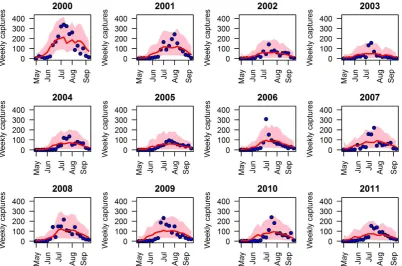
Model predictions associated with the estimated posterior distributions of model param-eters for the different seasons (from 2000 to 2011) were analyzed in terms of i) the weekly number of Cx. pipiens captured during the twenty-week survey period; ii) the total number of captured mosquitoes at the end of each year; iii) the highest weekly capture during each year; iv) the week at which the highest capture was observed; v) the start and the end of the mosquito season, defined as in Section 1.2 to be the weeks by which respectively 5% and 95% of the cumulative captures in the simulated season occurred; for clarity, from now on, we will denote these values by onset and offset; vi) the season length, defined as the number of weeks between the onset and the offset of the season (as in Section 1.2). The uncertainty surrounding model predictions is generated by both the variability of the estimated posterior distribution of free model parameters and the intrinsic stochasticity characterizing model simulation.

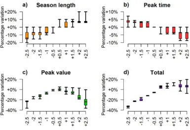
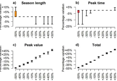
Finally, we applied the model to assess the influence of the temperature on the popu-lation dynamics. To this aim, we simulated each year ywith 10 different temperature patternsT(y,t) ranging fromT(y,t)−2.5◦toT(y,t)+2.5◦, where T(y,t) is the observed temporal pattern of temperature associated with year y. Following a similar approach, we investigated the role played by the larval carrying capacity by simulating each year

ywith different density-dependent factorsK, ranging from 0.5·K(y) to 1.5·K(y), where

K(y) is the estimated density-dependent factor for yeary.

2.3

Results and discussion

(37)

Eco-climatic drivers ofCx. pipiensdynamics 33

In agreement with collected data (see Figure 2.2c), our results show that the average cu-mulative number of trapped adults can substantially change between seasons, ranging from 510 (2.5-97.5% quantile predictions: 100-1887) in 2003 to 2425 (2.5-97.5% quantile predictions: 1194-4677) in 2000.

The highest capture is predicted to occur, on average, between the 27th and 31st week of the year (corresponding to the month of July) in good agreement with observed values (see Figure 2.2b). On the opposite, the predictions on the maximum number of trapped adults in a single capture session during the entire season are extremely variable among different simulations and do not accurately reproduce observed values. This field mea-sure is highly sensitive and reflects stochastic variations driven by site-specific factors such as rain and wind condition of the day. Indeed, strong wind and rainfalls might alterCx. pipiensdispersal and host-seeking behavior, possibly reducing the probability of being captured. In fact, data collected show that captures of two consecutive trapping sessions can be remarkably different (with differences sometimes of an order of magni-tude). In order to smooth the inherent variability in captures, we computed, for each trap, the 3-point moving average of weekly captures. The distribution of the maxima of moving averages, for each year, is shown in Figure 2.2d; it can be seen that the variabil-ity in model predictions is consistent (though a bit lower) with the observed variabilvariabil-ity among traps. In addition, years characterized by higher maximum number of trapped adults within a single capture are associated with higher peaks in model predictio