R E S E A R C H
Open Access
Chebyshev wavelets method for solving
Bratu’s problem
Changqing Yang
*and Jianhua Hou
*Correspondence: [email protected] Department of Science, Huaihai Institute of Technology,
Lianyungang, Jiangsu 222005, China
Abstract
A numerical method for one-dimensional Bratu’s problem is presented in this work. The method is based on Chebyshev wavelets approximates. The operational matrix of derivative of Chebyshev wavelets is introduced. The matrix together with the
collocation method are then utilized to transform the differential equation into a system of algebraic equations. Numerical examples are presented to verify the efficiency and accuracy of the proposed algorithm. The results reveal that the method is accurate and easy to implement.
1 Introduction
In this paper, we consider the boundary-value problem and initial value problem of Bratu’s problem. It is well known that Bratu’s boundary value problem in one-dimensional planar coordinates is of the form
u+λeu= , <x< , ()
with the boundary conditionsu() =u() = . Forλ> is a constant, the exact solution of equation () is given by []
u(x) = –ln
cosh(.θ(x– .))
cosh(.θ)
, ()
whereθ satisfies
θ=√λsinh(.θ). ()
The problem has zero, one or two solutions whenλ>λc,λ=λcandλ<λc, respectively,
where the critical valueλcsatisfies the equation
=
λccosh
θ
.
It was evaluated in [–] that the critical valueλcis given byλc= ..
In addition, an initial value problem of Bratu’s problem
u+λeu= , <x< , ()
with the initial conditionsu() =u() = will be investigated.
Bratu’s problem is also used in a large variety of applications such as the fuel ignition model of the thermal combustion theory, the model of thermal reaction process, the Chandrasekhar model of the expansion of the universe, questions in geometry and rel-ativity about the Chandrasekhar model, chemical reaction theory, radiative heat transfer and nanotechnology [–].
A substantial amount of research work has been done for the study of Bratu’s problem. Boyd [, ] employed Chebyshev polynomial expansions and the Gegenbauer as base functions. Syam and Hamdan [] presented the Laplace decomposition method for solving Bratu’s problem. Also, Aksoy and Pakdemirli [] developed a perturbation solution to Bratu-type equations. Wazwaz [] presented the Adomian decomposition method for solving Bratu’s problem. In addition, the applications of spline method, wavelet method and Sinc-Galerkin method for solution of Bratu’s problem have been used by [–].
In recent years, the wavelet applications in dealing with dynamic system problems, es-pecially in solving differential equations with two-point boundary value constraints have been discussed in many papers [, , ]. By transforming differential equations into alge-braic equations, the solution may be found by determining the corresponding coefficients that satisfy the algebraic equations. Some efforts have been made to solve Bratu’s problem by using the wavelet collocation method [].
In the present article, we apply the Chebyshev wavelets method to find the approximate solution of Bratu’s problem. The method is based on expanding the solution by Chebyshev wavelets with unknown coefficients. The properties of Chebyshev wavelets together with the collocation method are utilized to evaluate the unknown coefficients and then an ap-proximate solution to () is identified.
2 Chebyshev wavelets and their properties 2.1 Wavelets and Chebyshev wavelets
In recent years, wavelets have been very successful in many science and engineering fields. They constitute a family of functions constructed from dilation and translation of a single function called the mother waveletψ(x). When the dilation parameteraand the transla-tion parameterbvary continuously, we have the following family of continuous wavelets []:
ψa,b(x) =|a|–/ψ
x–b a
, a,b∈R,a= .
Chebyshev waveletsψn,m=ψ(k,n,m,x) have four arguments,n= , , . . . , k–,kcan
as-sume any positive integer,mis the degree of Chebyshev polynomials of first kind andx denotes the time.
ψn,m(x) = ⎧ ⎨ ⎩
αm√(k–)/ π Tm(
kx– n+ ), n– k–≤x<
n k–;
, otherwise, ()
where
αm= ⎧ ⎨ ⎩
√
, m= ;
andm= , , , . . . ,M– ,n= , , . . . , k–. HereT
m(x) are the well-known Chebyshev
poly-nomials of order m, which are orthogonal with respect to the weight functionω(x) = /√ –xand satisfy the following recursive formula:
T(x) = ,
T(x) =x,
Tm+(x) = xTm(x) –Tm–(x).
We should note that the set of Chebyshev wavelets is orthogonal with respect to the weight functionωn(x) =ω(kx– n+ ).
The derivative of Chebyshev polynomials is a linear combination of lower-order Chebyshev polynomials, in fact [],
⎧ ⎨ ⎩
Tm(x) = mm–k= Tk(x), meven;
Tm(x) = mm–k= Tk(x) +mT(x), modd.
()
2.2 Function approximation
A functionu(x) defined over [, ) may be expanded as
u(x) = ∞
n=
∞
m=
cnmψnm(x), ()
wherecnm= (u(x),ψnm(x)), in which (·,·) denotes the inner product with the weight
func-tionωn(x). Ifu(x) in () is truncated, then () can be written as
u(x)≈
k–
n= M–
m=
cnmψnm(x) =CTΨ(x), ()
whereCandΨ(x) are k–M× matrices given by
C= [c,c, . . . ,ck–]T,
Ψ(x) = [ψ,ψ, . . . ,ψk–]T
and
ci= [ci,ci, . . . ,ci,M–],
ψi(x) =
ψi(x),ψi(x), . . . ,ψi,M–(x)
, i= , , , . . . , k–.
3 Chebyshev wavelets operational matrix of derivative
In this section we first derive the operational matrixDof derivative which plays a great role in dealing with Bratu’s problem.
In the interval [(n– )/k–,n/k–),
ψn,m(x) =
αm(k–)/
√
π Tm
Applying () the derivative ofψn,m(x) is
ψn,m (x)
=
⎧ ⎨ ⎩
αm√(k–)/
π ·
k·mm–
k= Tk(kx– n+ ), meven;
αm√(k–)/
π ·
k·[mm–
k= Tk(kx– n+ ) +mT(kx– n+ )], modd.
The functionψi(x) is zero outside the interval [(i– )/k–,i/k–), so
ψi(x) =ψi(x)M, i= , , . . . , k–, ()
where
M= k·
⎛ ⎜ ⎜ ⎜ ⎜ ⎜ ⎜ ⎜ ⎜ ⎜ ⎝
√ √ √ · · · (M– )√ · · · · · · (M– )
..
. ... ... ... ... ... . .. ...
· · · (M– )
⎞ ⎟ ⎟ ⎟ ⎟ ⎟ ⎟ ⎟ ⎟ ⎟ ⎠
M×M
for evenM,
M= k·
⎛ ⎜ ⎜ ⎜ ⎜ ⎜ ⎜ ⎜ ⎜ ⎜ ⎝ √ √ √ · · · · · · · · · (M– )
..
. ... ... ... ... ... . .. ... · · · (M– )
⎞ ⎟ ⎟ ⎟ ⎟ ⎟ ⎟ ⎟ ⎟ ⎟ ⎠
M×M
for oddM.
In fact we have shown that
Ψ(x) =DΨ(x), ()
where
D=diagMT,MT, . . . ,MT.
From (), it can be generalized for anyn∈Nas
dnΨ(x) dxn =D
nΨ(x), n= , , , . . . . ()
4 Solution of Bratu’s problem
Consider Bratu’s problem given in (). In order to use Chebyshev wavelets, we first ap-proximateu(x) as
Applying () we can get
u(x) =CTDΨ(x).
Thus we have
CTDΨ(x) +λeCTΨ(x)= . ()
We now collocate () at k–M– points atx ias
CTDΨ(xi) +λeC
TΨ(x
i)= . ()
Suitable collocation points are
xi=
+cos
(i– )π
k–M–
, i= , , . . . , k–M– .
Thus with the boundary conditionsu() =u() = , we have
CTΨ() = , ()
CTΨ() = . ()
Equations (), () and () generate k–Mset of nonlinear equations. The approximate
solution of the vector C is obtained by solving the nonlinear system using the Gauss-Newton method.
5 Error analysis
Theorem . A function u(x)∈Lω([, ]),with bounded second derivative,say|u(x)| ≤
N,can be expanded as an infinite sum of Chebyshev wavelets,and the series converges uniformly to u(x),that is[],
u(x) = ∞
n=
∞
m=
cnmψnm.
Since the truncated Chebyshev wavelets series is an approximate solution of Bratu’s problem, so one has an error functionE(x) foru(x) as follows:
E(x) =u(x) –CTΨ(x).
The error bound of the approximate solution by using Chebyshev wavelets series is given by the following theorem.
Theorem . Suppose that u(x)∈Cm[, ]and CTΨ(x)is the approximate solution using
the Chebyshev wavelets method.Then the error bound would be obtained as follows:
E(x)≤
m!mm(k–)xmax∈[,]u m(x)
Proof Applying the definition of norm in the inner product space, we have
E(x)=
u(x) –CTΨ(x)dx.
Because the interval [, ] is divided into k–subintervalsI
n= [(n– )/k–,n/k–],n=
, , . . . , k–, then we can obtain
E(x)=
u(x) –CTΨ(x)dx
=
k–
k= n
k–
n– k–
u(x) –CTΨ(x)dt
≤
k–
k= n
k–
n– k–
u(x) –Pm(x)
dt,
wherePm(x) is the interpolating polynomial of degreemwhich agrees withu(x) at the
Chebyshev nodes onInwith the following error bound for interpolating [, ]:
u(x) –Pm(x)≤
m!mm(k–)maxx∈Inu m(x).
Therefore, using the above equation, we would get
E(x)≤
k–
k= n
k–
n– k–
u(x) –Pm(x)
dt
≤
k–
k= n
k–
n– k–
m!mm(k–)maxx∈Inu m(x)
dt
≤
k–
k= n
k–
n– k–
m!mm(k–)xmax∈[,]u m(x)
dt =
m!mm(k–)xmax∈[,]u m(x)
dt
=
m!mm(k–)xmax∈[,]u m(x)
.
6 Numerical examples
To illustrate the ability and reliability of the method for Bratu’s problem, some examples are provided. The results reveal that the method is very effective and simple.
Example . Consider the first case for Bratu’s equation as follows, whenλ= [, ]:
u+ eu= , <x< ,
u() =u() = .
()
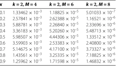
Table 1 Computed absolute errors for Example 6.1
x k=,M= k=,M= k=,M=
0.1 1.33462×10⁻³ 1.18825×10⁻⁵ 5.01033×10⁻⁷ 0.2 2.57841×10⁻³ 2.62388×10⁻⁵ 1.16521×10⁻⁶ 0.3 5.88781×10⁻³ 2.26840×10⁻⁵ 2.33696×10⁻⁶ 0.4 3.36183×10⁻³ 5.20260×10⁻⁵ 5.48713×10⁻⁶ 0.5 5.98507×10⁻³ 4.44306×10⁻⁵ 1.33512×10⁻⁶
0.6 3.59903×10⁻³ 2.53383×10⁻⁵ 2.40800×10⁻⁶
0.7 5.14675×10⁻³ 4.17100×10⁻⁵ 3.73327×10⁻⁶
0.8 1.43561×10⁻³ 3.25335×10⁻⁵ 7.18825×10⁻⁶
0.9 1.25962×10⁻³ 1.71598×10⁻⁵ 1.46832×10⁻⁶
between the absolute error of exact and approximate solutions for various values ofM (withk= ). Moreover, higher accuracy can be achieved by taking higher order approxi-mations.
Example . Consider the initial value problem [, –, ]
u– eu= , <x< ,
u() = , u() = .
()
The exact solution isu(x) = –ln(cos(x)). Here we solve it using Chebyshev wavelets, with k= ,M= . First we assume that the unknown functionu(x) is given by
u(x) =CTΨ(x).
Applying () we get
CTDΨ(xi) – eC
TΨ(x
i)= . ()
Using the initial condition, we obtain
CTΨ() = ,
CTDΨ() = .
()
Equations () and () generate a system of nonlinear equations. These equations can be solved for unknown coefficients of the vectorC. A comparison between the exact and the approximate solutions is demonstrated in Figure . From Figure , it can be found that the obtained approximate solutions are very close to the exact solution. In addition, Table shows the exact and approximate solutions using the method presented in Section and compares the results with the method presented in []. Also, by comparing the results of the table, we see that the results of the proposed method are more accurate.
7 Conclusions
Figure 1 Comparison of solutions for Example 6.2.
Table 2 Comparison of the results of the Chebyshev and Legendre wavelets method for Example 6.2
x Chebyshev wavelets Legendre wavelets Exact solutions
0.1 1.0016711×10⁻² 1.0016801×10⁻² 1.0016711×10⁻²
0.2 4.0269541×10⁻² 4.0269696×10⁻² 4.0269546×10⁻²
0.3 9.1383326×10⁻² 9.1382697×10⁻² 9.1383311×10⁻²
0.4 1.6445871×10⁻¹ 1.6444915×10⁻¹ 1.6445803×10⁻¹
0.5 2.6116111×10⁻¹ 2.6111176×10⁻¹ 2.6116848×10⁻¹
0.6 3.8339360×10⁻¹ 3.8367456×10⁻¹ 3.8393033×10⁻¹
0.7 5.3617551×10⁻¹ 5.3524690×10⁻¹ 5.3617151×10⁻¹
0.8 7.2271751×10⁻¹ 7.1991951×10⁻¹ 7.2278149×10⁻¹
0.9 9.5086960×10⁻¹ 9.4297240×10⁻¹ 9.5088488×10⁻¹
equations. Illustrative examples are included to demonstrate the validity and applicability of the technique.
Competing interests
The authors declare that they have no competing interests.
Authors’ contributions
CY completed the main study, carried out the results of this article and drafted the manuscript. JH checked the proofs and verified the calculation. All the authors read and approved the final manuscript.
Acknowledgements
Project is supported by the Huaihai Institute of Technology (No. Z2001151).
Received: 14 May 2013 Accepted: 16 May 2013 Published: 2 June 2013
References
1. Ascher, UM, Matheij, R, Russell, RD: Numerical Solution of Boundary Value Problems for Ordinary Differential Equations. SIAM, Philadelphia (1995)
2. Boyd, JP: Chebyshev polynomial expansions for simultaneous approximation of two branches of a function with application to the one-dimensional Bratu equation. Appl. Math. Comput.14, 189-200 (2003)
4. Hsiao, CH: Haar wavelet approach to linear stiff systems. Math. Comput. Simul.64, 561-567 (2004)
5. Buckmire, R: Application of a Mickens finite-difference scheme to the cylindrical Bratu-Gelfand problem. Numer. Methods Partial Differ. Equ.20(3), 327-337 (2004)
6. McGough, JS: Numerical continuation and the Gelfand problem. Appl. Math. Comput.89, 225-239 (1998) 7. Mounim, AS, de Dormale, BM: From the fitting techniques to accurate schemes for the Liouville-Bratu-Gelfand
problem. Numer. Methods Partial Differ. Equ.22(4), 761-775 (2006)
8. Syam, MI, Hamdan, A: An efficient method for solving Bratu equations. Appl. Math. Comput.176, 704-713 (2006) 9. Li, S, Liao, SJ: Analytic approach to solve multiple solutions of a strongly nonlinear problem. Appl. Math. Comput.169,
854-865 (2005)
10. Wazwaz, AM: Adomian decomposition method for a reliable treatment of the Bratu-type equations. Appl. Math. Comput.166, 652-663 (2005)
11. He, JH: Some asymptotic methods for strongly nonlinear equations. Int. J. Mod. Phys. B20(10), 1141-1199 (2006) 12. Boyd, JP: One-point pseudo spectral collocation for the one-dimensional Bratu equation. Appl. Math. Comput.217,
5553-5565 (2011)
13. Aksoy, Y, Pakdemirli, M: New perturbation iteration solutions for Bratu-type equations. Comput. Math. Appl.59, 2802-2808 (2010)
14. Caglara, H, Caglarb, N, Özer, M: B-spline method for solving Bratu’s problem. Int. J. Comput. Math.87(8), 1885-1891 (2010)
15. Jalilian, R: Non-polynomial spline method for solving Bratu’s problem. Comput. Phys. Commun.181, 1868-1872 (2010)
16. Venkatesh, SG, Ayyaswamy, SK, Raja Balachandar, S: The Legendre wavelet method for solving initial value problems of Bratu-type. Comput. Math. Appl.63, 1287-1295 (2012)
17. Rashidinia, J, Maleknejad, K, Taheri, N: Sinc-Galerkin method for numerical solution of the Bratu’s problem. Numer. Algorithms62, 1-11 (2013)
18. Lepik, U: Numerical solution of differential equations using Haar wavelets. Math. Comput. Simul.68(2), 127-143 (2005) 19. Daubechies, I: Ten Lectures on Wavelet. SIAM, Philadelphia (1992)
20. Sezer, M, Kaynak, M: Chebyshev polynomials solutions of linear differential equations. Int. J. Math. Educ. Sci. Technol.
27(4), 607-618 (1996)
21. Adibi, H, Assari, P: Chebyshev wavelet method for numerical solution of Fredholm integral equations of the first kind. Math. Probl. Eng.2010, 1-17 (2010)
22. Dahlquist, G, Björck, A: Numerical Methods in Scientific Computing, vol. 1. SIAM, Philadelphia (2008)
23. Biazar, J, Ebrahimi, H: Chebyshev wavelets approach for nonlinear systems of Volterra integral equations. Comput. Math. Appl.63(3), 608-616 (2012)
24. Batiha, B: Nnmerical solution of Bratu-type equations by the variational iteration method. Hacet. J. Math. Stat.39, 23-29 (2010)
doi:10.1186/1687-2770-2013-142
Cite this article as:Yang and Hou:Chebyshev wavelets method for solving Bratu’s problem.Boundary Value Problems