Extending the persistent primary variable algorithm to simulate non-isothermal two-phase two-component flow with phase change phenomena

(1)

R E S E A R C H

Open Access

Extending the persistent primary variable

algorithm to simulate non-isothermal

two-phase two-component flow with phase

change phenomena

Yonghui Huang

1,2†

, Olaf Kolditz

1,2

and Haibing Shao

1,3*†

*Correspondence: [email protected]

†_{Equal contributors}

1Helmholtz Centre for Environmental Research - UFZ, Permoserstr. 15, 04318 Leipzig, Germany

3Freiberg University of Mining and Technology, Gustav-Zeuner-Strasse 1, 09596 Freiberg, Germany Full list of author information is available at the end of the article

Abstract

In high-enthalpy geothermal reservoirs and many other geo-technical applications, coupled non-isothermal multiphase flow is considered to be the underlying governing process that controls the system behavior. Under the high temperature and high pressure environment, the phase change phenomena such as evaporation and condensation have a great impact on the heat distribution, as well as the pattern of fluid flow. In this work, we have extended the persistent primary variable algorithm proposed by (Marchand et al. Comput Geosci 17(2):431–442) to the non-isothermal conditions. The extended method has been implemented into the OpenGeoSys code, which allows the numerical simulation of multiphase flow processes with phase change phenomena. This new feature has been verified by two benchmark cases. The first one simulates the isothermal migration of H2through the bentonite formation in a waste repository. The second one models the non-isothermal multiphase flow of heat-pipe problem. The OpenGeoSys simulation results have been successfully verified by closely fitting results from other codes and also against analytical solution.

Keywords: Non-isothermal multiphase flow; Geothermal reservoir modeling; Phase change; OpenGeoSys

Background

In deep geothermal reservoirs, surface water seepages through fractures in the rock and moves downwards. At a certain depth, under the high temperature and pressure condition, water vaporizes from liquid to gas phase. Driven by the density difference, the gas steam then migrates upwards. Along with its path, it will condensate back into the liquid form and release its energy in the form of latent heat. Often, this multiphase flow process with phase transition controls the heat convection in deep geothermal reservoirs. Besides, such multiphase flow and heat transport are considered to be the underlying pro-cesses in a wide variety of applications, such as in geological waste repositories, soil vapor extraction of Non-Aqueous Phase Liquid (NAPL) contaminants (Forsyth and Shao 1991), and CO2capture and storage (Park et al. 2011; Singh et al. 2012). Throughout the process, different phase zones may exist under different temperature and pressure conditions. At lower temperatures, water flows in the form of liquid. With the rise of temperature, gas

(2)

and liquid phases may co-exist. At higher temperature, water is then mainly transported in the form of gas/vapor. Since the physical behaviors of these phase zones are different, they are mathematically described by different governing equations. When simulating the geothermal convection with phase change phenomena, this imposes challenges to the numerical models. To numerically model the above phase change behavior, there exist several different algorithms so far. The most popular one is the so-called primary vari-able switching method proposed by Wu and Forsyth (2001). In Wu’s method, the primary variables are switched according to different phase states. For instance, in the two phase region, liquid phase pressure and saturation are commonly chosen as the primary vari-ables; whereas in the single gas or liquid phase region, the saturation of the missing phase will be substituted by the concentration or mass fraction of one light component. This approach has already been adopted by the multiphase simulation code such as TOUGH (Pruess 2008) and MUFTE (Class et al. 2002). Nevertheless, the governing equations deduced from the varying primary variables are intrinsically non-differentiable and often lead to numerical difficulties. To handle this, Abadpour and Panfilov (2009) proposed the negative saturation method, in which saturation values less than zero and bigger than one are used to store extra information of the phase transition. Salimi et al. (2012) later extended this method to the non-isothermal condition, and also taking into account the diffusion and capillary forces. By their efforts, the primary variable switching has been successfully avoided. Recently, Panfilov and Panfilova (2014) has further extended the negative saturation method to the three-component three-phase scenario. As the nega-tive saturation value does not have a physical meaning, further extension of this approach to general multi-phase multi-component system would be difficult. For deep geothermal reservoirs, it requires the primary variables of the governing equation to be persistent throughout the entire spatial and temporal domain of the model. Following this idea, Neumann et al. (2013) chose the pressure of non-wetting phase and capillary pressure as primary variables. The two variables are continuous over different material layers, which make it possible to deal with heterogeneous material properties. The drawback of Neumann’s approach is that it can only handle the disappearance of the non-wetting phase, not its appearance. As a supplement, Marchand et al. (2013) suggested to use mean pressure and molar fraction of the light component as primary variables. This allows both of the primary variables to be constructed independently of the phase status and allows the appearance and disappearance of any of the two phases. Furthermore, this algorithm could be easy to be extended to multi-phases (≥3) multi-components (≥3) system.

(3)

verified against analytical solution and also against results from other numerical codes (Marchand et al. 2012). Furthermore, details of numerical techniques regarding how to solve the non-linear EOS system were discussed (‘Numerical solution of EOS’ section). In the end, general ideas regarding how to include chemical reactions into the current form of governing equations are introduced.

Method

Governing equations

Following Hassanizadeh and Gray (1980), we write instead the mass balance equations of each chemical component by summing up their quantities over every phase. According to Gibbs Phase Rule (Landau and Lifshitz 1980), a simplest multiphase system can be established with two phases and two components. Considering a system with water and hydrogen as constitutive components (with superscripthandw), they distribute in liquid and gas phase, with the subscriptα∈L,G. The component-based mass balance equations can be formulated as

∂(SLρLw+SGρGw) ∂t + ∇(ρ

w

LvL+ρ_GwvG)+ ∇(jwL+jwG)=Fw (1)

∂(SLρLh+SGρGh) ∂t + ∇(ρ

h

LvL+ρGhvG)+ ∇(jhL+jhG)=Fh, (2)

whereSLandSGindicate the saturation in each phase.ρ_αi (i ∈ {h,w},α ∈ {L,G}) repre-sents the mass density of i-component inαphase.refers to the porosity.FhandFware the source and sink terms. The Darcy velocityvLandvGfor each fluid phase are regulated by the general Darcy Law

vL= − KKrL

μL (∇

PL−ρLg) (3)

vG= − KKrG

μG (∇

PG−ρGg). (4)

Here,Kis the intrinsic permeability, andgrefers to the vector for gravitational force. The terms jw_L,jh_L,j_Gw, and jh_G represent the diffusive mass fluxes of each component in different phases, which are given by Fick’s Law as

j_α(i)= −S_αρ_αD_α(i)∇C_α(i). (5)

Here D(αi) is the diffusion coefficient, and Cα(i) the mass fraction. When the non-isothermal condition is considered, a heat balance equation is added, with the assumption that gas and liquid phases have reached local thermal equilibrium and share the same temperature.

∂[(1−SG)ρLuL+SGρGuG]

∂t +

(1−)∂(ρScST)

∂t (6)

+∇[ρGhGvG]+∇[ρLhLvL]−∇(λT∇T)

=QT+hvap

∂(ρLSL)

∂t − ∇(ρLvL)

(4)

pressure dependent. WhileρS andcS are the density and specific heat capacity of the soil grain,λT refers to the heat conductivity, andQT is source term,hvap(∂(ρL_∂_tSL) −

∇(ρLvL))represents the latent heat term according to (Gawin et al. 1995). Generally, the specific enthalpy in Eq. 6 can be described as follows

hα=cpαT. (7)

Herecpα is the specific heat capacity of phaseαat given pressure. At the same time, relationship between internal energy and enthalpy can be described as

h_α=u_α+P_αV_α, (8)

wherePα andVαare the pressures and volumes of phaseα. Since we consider the liquid phase is incompressible, its volume change can be ignored, i.e.h=u.

Non-isothermal persistent primary variable approach

Here in this work, we follow the idea of Marchand et al. (2013), where the ‘Persistent Primary Variable’ concept were adopted. A new choice of primary variables consists of:

• P [Pa] is the weighted mean pressure of gas and liquid phase, with each phase volume as the weighting factor. It depends mainly on the liquid saturationS.

P=γ (S)PG+(1−γ (S))PL (9)

Hereγ (S)stands for a monotonic function of saturation S, with

γ (S)∈[ 0, 1] ,γ (0)=0,γ (1)=1. In Benchmark I (‘Benchmark I: isothermal injection ofH2gas’ section), we choose

γ (S)=0

In Benchmark II (‘Benchmark II: heat pipe problem’ section), we choose

γ (S)=S2

When one phase disappears, its volume converges to zero, making theP value equal to the pressure of the remaining phase. If we assume the local capillary equilibrium, the gas and liquid phase pressure can both be derived based on the capillary pressure Pc, that is also a function of saturationS.

PL=P−γ (S)Pc(S) (10)

PG=P+(1−γ (S))Pc(S) (11)

• X [-] refers to the total molar fraction of the light component in both fluid phases. Similar to the mean pressureP, it is also a continuous function throughout the phase transition zones. We formulate it as

X= SNGX h

G+(1−S)NLXLh SNG+(1−S)NL

(12)

(5)

∂((SNG+(1−S)NL)X(i))

∂t (13)

+∇NLXL(i)vL+NGX_G(i)vG

+ ∇NLSLWL(i)+NGSGW_G(i)

=F(i)

withi∈(h,w)and the flow velocityv regulated by the generalized Darcy’s law, referred to Eqs. 3 and 4.

The molar diffusive flux can be calculated following Fick’s law

W_αi = −D(_αi)∇X_α(i). (14)

• T[ K]refers to the Temperature. If we consider the temperatureT as the third primary variable, the energy balance equation can then be included.

∂(1−SG)NLX_L(i)M(i)

uL+SGNGX(_Gi)M(i)

uG

∂t (15)

+(1−)∂(ρScST)

∂t − ∇

NG X_G(i)M(i)

hGvG

−∇NL X(Li)M(i)

hLvL

− ∇(λT∇T)=QT

The non-isothermal system can thus be simulated by the solution of combined Eqs. 13 and 15, withP, X, and T as primary variables. Once these three primary variables are determined, the other physical quantities are then constrained by them and can be obtained by the solution of EOS system. These secondary variables were listed in Table 1. Compared to the primary variable switching (Wu and Forsyth 2001) and the negative saturation (Abadpour and Panfilov 2009) approach, the choice ofPandXas primary vari-ables fully covers all three possible phase states, i.e., the single-phase gas, two-phase, and single-phase liquid regions. It also allows the appearance or disappearance of any of the two phases. Instead of switching the primary variable, the non-linearity of phase change behavior was removed from the global partial differential equations and was embedded into the solution of EOS.

Closure relationships

Mathematically, the solution for any linear system of equations is unique if and only if the rank of the equation system equals the number of unknowns. In this work, the com-bined mass conservation of Eqs. 1, 2, and the energy balance Eq. 6 must be determined by three primary variables. Other variables are dependent on them and considered to be secondary. Such nonlinear dependencies form the necessary closure relationships.

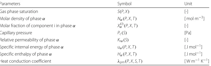
Table 1List of secondary variables and their dependency on the primary variables

Parameters Symbol Unit

Gas phase saturation S(P,X) [-]

Molar density of phase_α N_α₍P,X,T₎ [ mol m−3]

Molar fraction of component i in phase_α X_α(i)₍P,X,T₎ [-]

Capillary pressure Pc(S) [Pa]

Relative permeability of phaseα Krα(S) [-]

(6)

Constitutive laws

Dalton’s Lawregulates that the total pressure of a gas phase is equal to the sum of partial pressures of its constitutive non-reacting chemical component. In our case, a gas phase with two components, i.e., water and hydrogen is considered. Then the gas phase pressure

PGwrites as

PG=Ph_G+Pw_G. (16)

Ideal Gas LawIn our model, the ideal gas law is assumed, where the response of gas phase pressure and volume to temperature is regulated as

PG= nRT

V , (17)

whereRis the Universal Gas Constant (8.314 J mol−1K−1),V is the volume of the gas andnstands for the mole number gas. Reorganizing the above equation gives the molar density of gas phaseNG

NG= n

V =

PG

RT. (18)

Combining Dalton’s Law of Eq. 16, we have

N_Gh = P h G RT,N

w G =

P_Gw

RT. (19)

Furthermore, the molar fraction of componenti can be obtained by normalizing its partial pressure with the total gas phase pressure,

Xi_G= P i G PG

. (20)

Incompressible FluidUnlike the gas phase, the liquid phase in our model is consid-ered to be incompressible, i.e., the density of the fluid is linearly dependent on the molar amount of the constitutive chemical component. By assuming standard water molar den-sityN_Lstd = ρstdw

Mw, withρ_wstdrefers to the standard water mass density (1000 kg m−3in our model), the in-compressibility of the liquid phase writes as

NL= N_Lstd

1−X_Lh. (21)

Henry’ LawWe assume that the distribution of light component (hydrogen in our case) can be regulated by the Henry’s coefficientH_Wh (T), which is a temperature-dependent parameter.

P_GhH_Wh (T)=NLXLh (22)

Raoult’s LawFor the heavy component (water), we apply Raoult’s Law that the partial pressure of the water component in the gas phase changes linearly with its molar fraction in the liquid.

P_Gw=X_LwPw_Gvapor(T) (23)

HereX_Lwis the molar fraction of the water component in the liquid phase.Pw_Gvapor(T)

is the vapor pressure of pure water, and it is a temperature-dependent function in non-isothermal scenarios.

(7)

X_LhN_Lstd X_LwH_Wh (T) +X

w

LPGvaporw (T)=PG (24)

PGXhG= N_Lstd H_Wh(T)

X_Lh

X_Lw (25)

According to Eqs. 24 and 25, X_Lh and X_Gh can be calculated explicitly, under the condition:

G(T)= H h

W(T)PGvaporw (T)

N_Lstd <

1

4 (26)

which is obviously satisfied in water-air and water-hydrogen system, i.e., under the con-dition that the temperature T is 25◦C, with H_Wh(T) = 7.8 × 10−6[ mol m−3Pa−1],

P_Gvaporw (T) = 3173.07[ Pa], then we could haveG(T) = 4.54×10−7 1₄. Here, if we only consider isothermal condition, the temperature is assumed to be fixed withT0. In summary,X_LhandX_Ghcould be expressed as:

X_Lh=Xm(PL,S,T0)=

N_Lstd+(PL+Pc)HWh (T0) 2H_Wh(T0)P_Gvaporw (T0)

(27)

+

(N_Lstd+(PL+Pc)H_Wh (T0))2−4(PL+Pc)H_Wh (T0)N_LstdP_Gvaporw (T0)

2H_Wh (T0)P_Gvaporw (T0)

X_Gh =XM(PG,S,T0)=

X_LhN_Lstd H_Wh (T0)PG(1−XLh)

(28)

WhereSis the saturation of light component, andPcrepresents the capillary pressure. The above equations are the most general way of calculating the distribution of molar fraction. In Benchmark I (‘Benchmark I: isothermal injection of H2gas’ section), we follow Marchand’s idea (Marchand and Knabner 2014), by assuming there is no water vaporiza-tion and the gas phase contains only hydrogen, which indicatePG ≡ Ph_GandX_Gh ≡ 1. Therefore Eqs. 27 and 28 could be reformulated as:

X_Lh=Xm(PL,S,T0)= (

PL+Pc)H_Wh (T0) (PL+Pc)H_Wh(T0)+N_Lstd

(29)

X_Gh ≡1 (30)

Here, for simplification purpose, if we combined with Eqs. 10 and 11,Xh_LandXh_Gcould be expressed as functions of mean pressurePand gas phase saturationS, and the above formulation can be transformed to

X_Lh=Xm(PL(P,S(P,X)),S(P,X),T0)=Xm(P,S,T0) (31)

X_Gh =XM(PG(P,S(P,X)),S(P,X),T0)=XM(P,S,T0). (32)

(8)

• In two phase region

Molar fraction of hydrogen (X_LhandX_Gh) and molar density in each phase (NGand NL) are all secondary variables that are dependent on the change of pressure and saturation. They can be determined by solving the following non-linear system.

X_Lh=Xm(P,S,T0) (33)

X_Gh =XM(P,S,T0) (34)

NG=

PG(P,S) RT0

(35)

NL= N_Lstd

1−X_Lh (36)

SNG(X−XhG)+(1−S)NL(X−XLh)

SNG+(1−S)NL =

0 (37)

• In the single liquid phase region

In a single liquid phase scenario, the gas phase does not exist, i.e., the gas phase saturationS always equals to zero. Meanwhile, the molar fraction of light component in the gas phaseXh_Gcan be any value, as it will be multiplied with the zero saturation (see Eqs. 13 to 14) and vanish in the governing equation. This also applies to the gas phase molar densityNG, whereas the two parameters can be arbitrarily given, and have no physical impact. So to determine the EOS, we only need to solve for the liquid phase molar fraction and density.

X_Lh=X (38)

NL= N_Lstd

1−X (39)

• In the single gas phase region

Similarly, in a single gas phase scenario, the liquid phase does not exist, i.e., the gas phase saturationS always equals to 1, whereas the liquid phase saturation remains zero. Meanwhile, the molar fraction of light component in the liquid phaseX_Lhcan be any value, as it will be multiplied with the zero liquid phase saturation (see Eqs. 13 to 14) and vanish in the governing equation. This also applies to the liquid phase molar densityNG, whereas the two parameters can be arbitrarily given, and have no physical meaning. So to determine the EOS, we only need to solve for the gas phase molar fraction and density.

X_Gh =X

NG= P RT0

EOS for non-isothermal systems

(9)

a non-isothermal transport, high non-linearity of the model exists in the complex varia-tional relationships between secondary variables and primary variables. Therefore, how to set up an EOS system for each fluid is a big challenge for the non-isothermal multi-phase modeling. In the literature, (Class et al. 2002; Olivella and Gens 2000; Peng and Robinson 1976; Singh et al. 2013a, and Singh et al. 2013b) have given detailed procedures of solving EOS to predicting the gas and liquid thermodynamic and their transport prop-erties. Here in our model, we follow the idea by Kolditz and De Jonge (2004). Detailed procedure regarding how to calculate the EOS system is discussed in the following.

Vapor pressure As we discussed in the ‘Constitutive laws’ section, vapor pressure is a key parameter for determining the molar fractions of different components in each phase. The equilibrium restriction on vapor pressure of pure water is given by Clausius-Clapeyron equation (Çengel and Boles 1994).

Pw_Gvapor(T)=P0exp

1

T0 − 1

T

hw_GMw R

(40)

wherehw_Gis enthalpy of vaporization,Mwis molar mass of water.P0represents the vapor pressure of pure water at the specific TemperatureT0. In our model, we chooseT0 = 373K,P0=101, 325Pa. An alternative method is using the Antoine equation, written as

log10(PwGvapor(T))=A− B

C+T (41)

with A, B, and C as the empirical parameters. Details regarding this formulation can be found in Class et al. (2002).

Specific enthalpySpecific enthalpyhα[J mol−1] is the enthalpy per unit mass. Accord-ing to Eq. 6, we need to know the specific enthalpy of a certain phase. In particular, since component-based mass balance is considered, we calculate the phase enthalpy as the sum of mole (mass) specific enthalpy of each component in this phase. Here we assume that the energy of mixing is ignored. For instance, the water-air system applied in the second benchmark is formulated as

hG=hairG XGair+h wvap

G X

wvap

G (42)

hL=hairL XLair+h wliq

L X

wliq

L (43)

Herehair_G is the specific enthalpy of air in gas phase,hw_Gvapis specific enthalpy of vapor water in gas phase,hair_L represents the specific enthalpy of the air dissolved in the liquid phase, whilehw_Lliq donates the specific enthalpy of the liquid water in liquid phase. While

Xair_G ,X_Gwvap,X_LairandX_Lwliqrepresent molar fraction [-] of each component (air and water) in the corresponding phase (gas and liquid).

Henry coefficientWe assume Henry’s Law is valid under the non-isothermal condition. Therefore Henry coefficient is a secondary variable. In the water-air system, it can be defined as (Kolditz and De Jonge 2004)

H_Wh(T)=(0.8942+1.47 exp(−0.04394T))×10−10 (44)

withTthe temperature value in◦C.

(10)

λpm=λSpmL=SG=0+

SL(λSpmL=1−λSpmL=0)+

SG(λSpmG=1−λSpmG=0) (45)

FugacityWhen the thermal equilibrium is reached, the chemical potentials of compo-nentiin gas and liquid phase equal with each other. This equilibrium relationship can be formulated as the equation of chemical potentialν

ν(i) G(PG,X

(i) L ,X(

i) G,T)=ν

(i) L

PL,XL(i),X( i) G,T

In our model, the fugacity was applied instead of chemical potential. The above relationship is then transformed to the equivalence of component fugacities, where

f_G(i)=f_L(i)

holds for each component i in each phase. In order to compute the fugacity of a component in a particular phase, the following formulation is used

f_α(i)=PαX_α(i)φ_α(i) (46)

whereφ_α(i)is the respective fugacity coefficient of component.

Numerical scheme Numerical solution of EOS Physical constraints of EOS

Since the pore space should be fully occupied by either or both the gas and liquid phases, the sum of phase saturation should equal to one. By definition, the saturation for each phase should be no less than zero and no larger than one. This constraint is summarized as

α

Sα =1 ∧ Sα>0 (α∈G,L) (47)

Similarly, the sum of the molar fraction for all components in a single phase should also be in unity, and this second constraint can be formulated as

i

X_G(i)=1 ∧ i

X(_Li)=1 with X_G(i)>0 ∧ X(_Li)>0 (i∈h,w) (48)

Combining these constraints, we have

S=0∧X_Lh≤Xm(P, 0,T) (49)

0≤S≤1∧Xm(P,S,T)−XLh=0,XhG−XM(P,S,T)=0 (50)

S=1∧X_Gh ≥XM(P, 1,T) (51)

For the Eqs. 49 to 51, they contain both equality and inequality relationships, which impose challenges for the numerical solution. In order to solve it numerically, we intro-duce a minimum function (Kanzow 2004; Kräutle 2011), to transform the inequalities. It is defined as

Ψ (a,b):=min{a,b} (52)

Combined with Eqs. 49 to 51, they can be transformed to

(11)

(1−S,X_Gh−XM(P,S,T))=0 (54)

SNG(X−X_Gh)+(1−S)NL(X−XLh)

SNG+(1−S)NL =

0 (55)

Then Eqs. 53 to 55 formulates the EOS system, which needs to be solved on each mesh node of the model domain.

Numerical scheme of solving EOS

For the EOS, the primary variablesPandXare input parameters and act as the external constraint. The saturationS, gas and liquid phase molar fraction of the light component

Xh_GandXh_Lare then the unknowns to be solved. Once they have been determined, other secondary variables can be derived from them. When saturation is less than zero or big-ger than one, the second argument of the minimization function in Eq. 53 will be chosen. Then it effectively prevents the saturation value from moving into unphysical value. This transformation will result in a local Jacobian matrix that might be singular. Therefore, a pivoting action has to be performed before the Jacobian matrix is decomposed to cal-culating the Newton step. An alternative approach to handle this singularity is to treat the EOS system as a nonlinear optimization problem with the inequality constraints. Our tests showed that the optimization algorithms such as Trust-Region method are very robust in solving such a local problem, but the calculation time will be considerably longer, compared to the Newton-based iteration method.

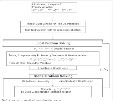
Numerical solution of the global equation system

In this work, we solve the global governing equation Eqs. 13 to 15 with all the closure relationships simultaneously satisfied. To handle the non-linearities, a nested Newton scheme was implemented (see the flow chart in Fig. 1). All the derivatives in the EOS sys-tem Eqs. 53 to 55 are computed exactly and the local Jacobian matrix is constructed in an analytical way, while the global Jacobian matrix is numerically evaluated based on the finite difference method. For the global equations, the time was discretized with the back-ward Euler scheme, and the spatial discretization was performed with the Galerkin Finite Element method. In each global Newton iteration, the updated global variablesP,X, and

Tfrom the previous iteration were passed to the EOS system, and acted as constraints to solve for secondary variables. The solution of Eqs. 53 to 55 was performed one after the other on each mesh node of the model domain.

For Newton iterations, the following convergence criteria was applied.

Residual(Step(k))₂≤ (56)

where2denotes the Euclidean norm. A tolerance value=1×10−14were adopted for the EOS and 1×10−9for the global Newton iterations.

Handling unphysical values during the global iteration

(12)

Fig. 1Scheme of the algorithm for global equation system

definition of the physical variables such asNG,NLforX <0, as was done in (Marchand et al. 2013), (Marchand and Knabner (2014), and (Abadpour and Panfilov 2009). In our implementation, we chose an alternative and more straightforward method, which is adding a damping factor in each global Newton iteration when updating the unknown vector. The damping factorδare chosen as follows,

1

δ =max{1, 2∗ P(j)

P(j) , 2∗

X(j) X(j) , 2∗

T(j)

T(j) } (57)

whereP(j),X(j)andT(j)denote pressure/molar fraction/temperature at nodej.

Results and Discussions

(13)

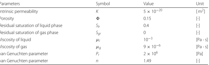
Benchmark I: isothermal injection of H2gas

The background of this benchmark is the production of hydrogen gas due to the corro-sion of the metallic container in the nuclear waste repository. Numerical model is built to illustrate such gas appearance phenomenon. The model domain is a two-dimensional hor-izontal column representing the bentonite backfill in the repository tunnel, with hydrogen gas injected on the left boundary. This benchmark was proposed in the GNR MoMaS project by French National Radioactive Waste Management Agency. Several research groups has made contributions to test the benchmark and provided their reference solu-tions (Ben Gharbia and Jaffré 2014; Bourgeat et al. 2009; Marchand and Knabner 2014; Neumann et al. 2013). Here we adopted the results proposed in Marchand’s paper Marchand and Knabner 2014 for comparison.

Physical scenario

Here a 2D rectangular domain =[ 0, 200]×[−10, 10] m (see Fig. 2) was considered with an impervious boundary at imp =[ 0, 200]×[−10, 10] m, an inflow boundary at in = {0}×[−10, 10] m, and an outflow boundary atout = {200}×[−10, 10] m. The domain was initially saturated with water, hydrogen gas was injected on the left-hand-side boundary within a certain time span ([ 0, 5×104century]). After that the hydrogen injection stopped and no flux came into the system. The right-hand-side boundary is kept open throughout the simulation. The initial condition and boundary conditions were summarized as

• X(t=0)=10−5 and PL(t=0)=PoutL =106[ Pa]on.

• qw_·_ν₌_qh_·_ν₌₀_on imp.

• qw·ν=0,qh·ν=Qh_d=0.2785 [ mol century−1m−2]onin.

• X=0andPl=PLout=106[ Pa]onout.

Model parameters and numerical settings

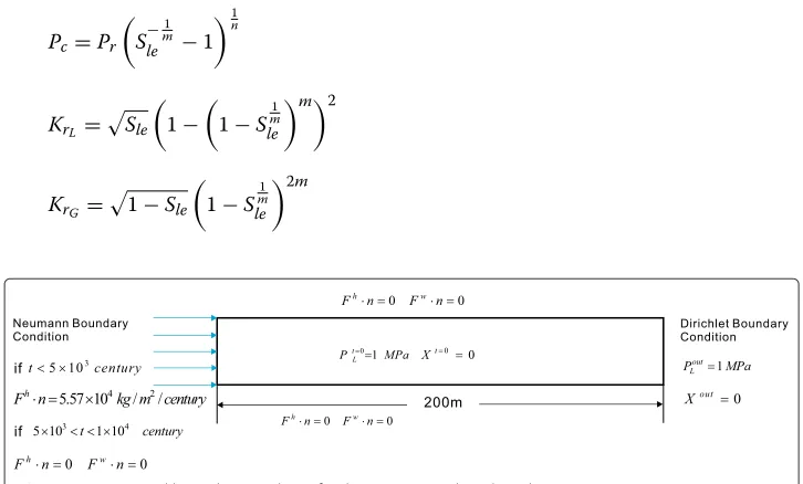
The capillary pressure Pc and relative permeability functions are given by the van-Genuchten model (Van Genuchten 1980).

Pc=Pr

S−

1

m le −1

1

n

KrL=

S_le

1−

1−Sm1 le

m2

KrG =

1−Sle

1−S

1

m le

2m

(14)

where m = 1 − 1_n, Pr andn are van-Genuchten model parameters and the effective saturationSleis given by

Sle=

1−Sg−Slr 1−Slr−Sgr

(58)

hereSlr andSgr indicate the residual saturation in liquid and gas phases, respectively. Values of parameters applied in this model are summarized in Table 2.

We created a 2D triangular mesh here with 963 nodes and 1758 elements. The mesh element size varies between 1m and 5m. A fixed time step size of 1 century is applied. The entire simulated time from 0 to 104_{centuries were simulated. The entire execution time} is around 3.241×104s.

Results and analysis

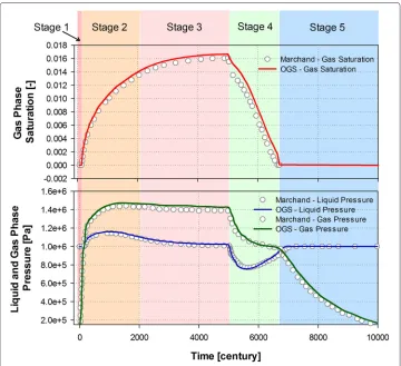
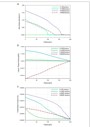
The results of this benchmark are depicted in Fig. 3. The evolution of gas phase satura-tion and the gas/liquid phase pressure at the inflow boundaryin over the entire time span are shown. In additional, we compare results from our model against those given in Marchand’s paper (Marchand and Knabner 2014). In Fig. 3, solid lines are our simula-tion results while the symbols are the results from Marchand et al. It can be seen that a good agreement has been achieved. Furthermore, the evolution profile of the gas phase saturationSg, the liquid phase pressurePL, and the total molar fraction of hydrogenX are plotted at different time (t = 150, 1×103, 5×103, 6×103centuries) in Fig. 4a−c, respectively.

By observing the simulated saturation and pressure profile, the complete physical process of H2injection can be categorized into five subsequent stages.

1) The dissolution stage: After the injection of hydrogen at the inflow boundary, the gas first dissolved in the water. This was reflected by the increasing concentration of hydrogen in Fig. 4c. Meanwhile, the phase pressure did not vary much and was kept almost constant (see Fig. 4b).

2) Capillary stage: Given a constant temperature, the maximal soluble amount of H2 in the water liquid is a function of pressure. In this MoMaS benchmark case, our simula-tion showed that this threshold value was about 1×10−3mol H2per mol of water at a pressure of 1×106_{[Pa]. Once this pressure was reached, the gas will emerge and formed} a continuous phase. As shown in Fig. 4a, at approximately 150 centuries, the first phase transition happens. Beyond this point, the gas and liquid phase pressure quickly increase, while hydrogen gas is transported towards the right boundary driven by the pressure and concentration gradient. In the meantime, the location of this phase transition point also slowly shifted towards the middle of the domain.

Table 2Fluid and porous medium properties applied in the H2migration benchmark

Parameters Symbol Value Unit

Intrinsic permeability K 5×10−20 [ m2_]

Porosity 0.15 [-]

Residual saturation of liquid phase Slr 0.4 [-]

Residual saturation of gas phase Sgr 0 [-]

Viscosity of liquid μl 10−3 [Pa·s]

Viscosity of gas μg 9×10−6 [Pa·s]

van Genuchten parameter Pr 2×106 [Pa]

(15)

Fig. 3Evolution of pressure and saturation over time

3) Gas migration stage: The hydrogen injection process continued until the 5000th century. Although the gas saturation continues to increase, pressures in both phases begin to decline due to the existence of the liquid phase gradient. Eventually, the whole system will reach steady state with no liquid phase gradient.

4) Recovery stage: After hydrogen injection was stopped at the 5000th century, the water came back from the outflow boundary towards the left, which was driven by the capillary effect to occupy the space left by the disappearing gas phase. During this stage, the gas phase saturation begins to decline, and both phase pressures drop even below the initial pressure. The whole process will not stop until the gas phase completely disappeared.

5) Equilibrium stage: After the complete disappearance of the gas phase, the satura-tion comes to zero again, and the whole system will reach steady state, with pressure and saturation values same as the ones given in the initial condition.

Benchmark II: heat pipe problem

(16)

Fig. 4Evolution of (a) gas phase saturation, (b) liquid phase pressure, and (c) total hydrogen molar fraction over the whole domain at different time

(17)

are listed in Table 3. Interested readers may also refer to the supplementary material regarding how this solution was deducted (see Additional file 1-6).

Physical scenario

As shown in Fig. 5, the heat pipe was represented by a 2D horizontal column (2.25 m in length and 0.2 m in diameter) of porous media, which was partially saturated with a liquid phase saturation value of 0.7 at the beginning. A constant heat flux (QT =100 [ W m−2]) was imposed on the right-hand-side boundaryin, representing the continuously operat-ing heatoperat-ing element. At the left-hand-side boundaryout, Dirichlet boundary conditions were imposed for TemperatureT =70◦C, liquid phase pressurePG=1×105[ Pa], effec-tive liquid phase saturationSle = 1, and air molar fraction in the gas phaseXGa = 0.71. Detailed initial and boundary condition are summarized as follows.

• P(t=0)=1×105[ Pa], SL(t=0)=0.7, T(t=0)=70 [◦C] on the entire domain.

• qw·ν=qh·ν=0 onimp.

• qw_·_ν₌_qh_·_ν₌_0, _qT_·_ν₌_Q

T onin.

• P=1×105[ Pa], SL=0.7,T=70 [◦C] onout.

Model parameters and numerical settings

For the capillary pressure−saturation relationship, van Genuchten model was applied. The parameters used in the van Genuchten model are listed in Table 3. The water−air relative permeability relationships were described by the Fatt and Klikoffv formulations (Fatt and Klikoff Jr 1959).

KrG =(1−Sle)3 (59)

KrL =S_le3 (60)

whereSleis the effective liquid phase saturation, referred to Eq. 58.

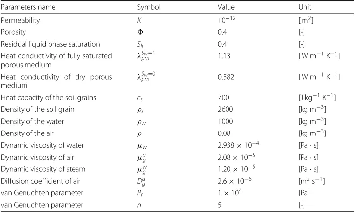
Table 3Parameters applied in the heat pipe problem

Parameters name Symbol Value Unit

Permeability K 10−12 [ m2_]

Porosity 0.4 [-]

Residual liquid phase saturation Slr 0.4 [-]

Heat conductivity of fully saturated porous medium

λSw=1

pm 1.13 [ W m−1K−1]

Heat conductivity of dry porous

medium λ

Sw=0

pm 0.582 [ W m−1K−1]

Heat capacity of the soil grains cs 700 [J kg−1K−1]

Density of the soil grain ρs 2600 [kg m−3]

Density of the water ρw 1000 [kg m−3]

Density of the air _ρ 0.08 [kg m−3]

Dynamic viscosity of water _μw 2.938×10−4 [Pa·s]

Dynamic viscosity of air μa_g 2.08×10−5 [Pa·s] Dynamic viscosity of steam μw

g 1.20×10−5 [Pa·s]

Diffusion coefficient of air Da

g 2.6×10−5 [m2s−1]

van Genuchten parameter Pr 1×104 [Pa]

(18)

Fig. 5Geometry of the heat pipe problem

We created a 2D triangular mesh here with 206 nodes and 326 elements. The averaged mesh element size is around 6m. A fixed size time stepping scheme has been adopted, with a constant time step size of 0.01 day. The entire simulated time from 0 to 104_day were simulated.

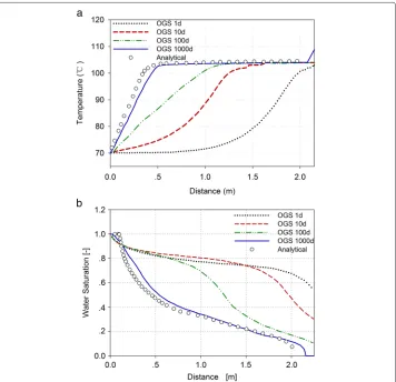
Results

The results of our simulation were plotted along the central horizontal profile over the model domain at y = 0.1 m, and compared against semi-analytical solution. Tempera-ture and saturation profiles at day 1, 10, 100, 1000 are depicted in Fig. 6a, b respectively. As the heat flux was imposed on the right-hand-side boundary, the temperature kept rising there. After 1 day, the boundary temperature already exceeded 100◦C, and the water in the soil started to boil. Together with the appearance of steam, water saturation

(19)

on the right-hand-side began to decrease. After 10 days, the boiling point has almost moved to the middle of the column. Meanwhile, the steam front kept boiling and shifted to the left-hand-side, whereas liquid water was drawn back to the right. After about 1000 days, the system reached a quasi-steady state, where the single phase gas, two phase and single phase liquid regions co-exist and can be distinguished. A pure gas phase region can be observed on the right and liquid phase region dominates the left side.

Discussion

Analysis of the differences in benchmark II

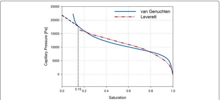
From Fig. 6a, b, some differences can still be observed in comparison to the semi-analytical solution. Our hypothesis is this difference originates from the capillary pressure−saturation relationship adopted in our numerical implementation. In the orig-inal formulation of Udell and Fitch (1985), the Leverett model was applied to produce the semi-analytical solution. It is assumed that the liquid and gas are immiscible and thus there is no gas component dissolved in the liquid phase, and vice versa. In our work, we cannot precisely follow the same assumption, since the dissolution of chemi-cal component in both phases is a requirement for the chemi-calculation of phase equilibrium. When considering phase change, we need to allow the saturationSto drop below the residual saturation, so that the evaporation as well as the condensation process can occur. In the traditional van Genuchten model, infinite value of capillary pressure may occur in the lower residual saturation region. Therefore we have made regularization that allows water saturation to fall below the residual saturation, as demonstrated in Fig. 7. Every time the capillary pressure needs to be evaluated, an if-else judgment is performed.

ifSlr<S<1then

¯

Pc(S)=Pc(S)

(61)

else

if0<S<Slrthen

¯

Pc(S)=Pc(Slr)−Pc(Slr)(S−Slr)

(62)

end end

(20)

Fig. 7The regularization of the van Genuchten model

Continuity of the global system and convergence of the iteration

In this work, we have only considered the homogeneous medium, where the primary variables ofP andXare always continuous over the entire domain. For some primary variables, their derivatives in the governing Eqs. (13)−(15) are discontinuous at locations where the phase transition happens, i.e.,X = Xm(P,S = 0,T) andX = XM(P,S = 1,T). For instance, _∂∂_XS and_∂∂_PS might produce singularities atS= 0 andS =1, and they can cause trouble on the conditioning of the global Jacobian matrix. In our simulation, a damped Newton iterations with line search has been adopted (see the ‘Handling unphys-ical values during the global iteration’ section). We observed that such derivative terms will result in an increased number of global Newton iterations, and the linear iteration number to solve the Newton step as well. It does not alter the convergence of the Newton scheme, as long as the function is Lipschitz continuous.

We are aware of the fact that this issue may be more difficult to handle for the het-erogeneous media, where the primary variablePandXcould not be directly applied any more because of the non-continuity over the heterogeneous interface (Park et al. 2011). In that case, choosing the primary variables which are continuous over any interface of the medium is a better option. Based on the analysis by Ern and Mozolevski (2012), if we assume Henry’s law is valid, concentration, or in another word, the molar or mass fraction of the hydrogen in the liquid phaseρ_Lh(X_Lh), gas/liquid phase pressurePG/PL, as well as the capillary pressure are all continuous over the interface. Therefore, they are the poten-tial choices of primary variable which can be applied in the heterogeneous media (see (Angelini et al. 2011); (Neumann et al. 2013), and (Bourgeat et al. 2013)). We are currently investigating these options and will report on the results in subsequent work.

Conclusions

(21)

• For the GNR MoMaS (Bourgeat et al. 2009) benchmark (‘Benchmark I: isothermal injection ofH2gas’ section), the extended model is capable of simulating the migration ofH2gas including its dissolution in aqueous phase. The simulated results fitted well with those from other codes (Marchand et al. 2013; Marchand and Knabner 2014).

• For the non-isothermal benchmark, we simulated the heat pipe problem and verified our result against the semi-analytical solution (‘Benchmark II: heat pipe problem’ section). Furthermore, our numerical model extended the original heat pipe problem to include the phase change behavior.

Currently, we are working on the incorporation of equilibrium reactions, such as the mineral dissolution and precipitation, into the EOS system. As our global mass-balance equations are already component based, one governing equation can be written for each basis component. Pressure, temperature, and molar fraction of the chemical components can be chosen as primary variables. Inside the EOS problem, the amount of secondary chemical components can be calculated based on the result of basis, which can further lead to the phase properties as density and viscosity. The full extension of including temperature-dependent reactive transport system will be the topic of a separate work in the near future.

Nomenclature

Greek symbols

Tolerance value for Newton iteration. [-]

λT Heat Conductivity. [W m−1K−1]

μα Viscosity inαphase. [Pa·s]

νi

α Chemical potential of i-component inαphase. [Pa]

Porosity. [-]

φi

α fugacity coefficient of i-component inαphase. [-]

ρi

α Mass density of i-component inαphase. [Kg m−3]

Operators

∧ Logical "and"

2 Euclidean norm

Ψ (a,b) Minimum function

Roman symbols

g Vector for gravitational force. [m s−2_]

cpα Specific heat capacity in phaseαat given pressure. [J Kg−1K−1] cS Specific heat capacity of soil grain. [J Kg−1K−1] Di_α Diffusion coefficient of i-component in phaseα. [m2s−1] Fi _{Mass source/sink term for i-component.} _{[Kg m}−3_s−1_]

f_αi Fugacity of i-component inαphase. [Pa]

Hh

W Henry coefficient. [mol Pa−1m−3]

hα Specific enthalpy. [J Kg−1]

ji

α Diffusive mass flux of i-component inαphase. [mol m−2s−1]

K Intrinsic Permeability. [m2]

Nα Molar density inαphase. [mol m−3_]

Pα Pressure inαphase. [Pa]

Pw

Gvapor Vapor pressure of pure water. [Pa]

Pc Capillary pressure. [Pa]

(22)

R Universal Gas Constant. [J mol−1K−1]

Sαr Residual saturation inαphase. [-]

Sα Saturation inαphase. [-]

Sle Effective saturation. [-]

T Temperature. [K]

uα Specific internal energy. [J Kg−1]

Vα Volume inαphase. [m3]

vα Darcy velocity inαphase. [m s−1]

X Total molar fraction of light component in two phases. [-]

X_αi Molar Fraction of i-component inαphase. [-]

Additional files

Additional file 1: This document introduces how this analytical solution is deducted.

Additional file 2: This is the main matlab script file, which will be executed to produce the analytical solution. Additional file 3: This file constructs the four coupled differential equations.

Additional file 4: This file calculates the relative permeability of gas phase. Additional file 5: This file calculates the relative permeability of liquid phase.

Additional file 6: This file calculates the capillary pressure, with water saturation as the input parameter.

Competing interests

The authors declare that they have no competing interests. Authors’ contributions

YH implemented the extended method into the OpenGeoSys software, produced simulation results of the two benchmarks, and also drafted this manuscript. HS designed the numerical algorithm of solving the coupled PDEs, and also contributed to the code implementation. OK coordinated the development of OpenGeoSys, and contributed to the manuscript writing. All authors read and approved the final manuscript.

Acknowledgements

We would thank to Dr. Norihito Watanabe for his thoughtful scientific suggestions and comments on this paper. This work has been funded by the Helmholtz Association through the program POF III-R41 ‘Geothermal Energy Systems’. The first author would also like to acknowledge the financial support from Chinese Scholarship Council (CSC).

Author details

1_{Helmholtz Centre for Environmental Research - UFZ, Permoserstr. 15, 04318 Leipzig, Germany.}2_{Technical University of}

Dresden, Helmholtz-Strane 10, 01062 Dresden, Germany.3_{Freiberg University of Mining and Technology,}

Gustav-Zeuner-Strasse 1, 09596 Freiberg, Germany. Received: 17 December 2014 Accepted: 7 May 2015

References

Abadpour A, Panfilov M (2009) Method of negative saturations for modeling two-phase compositional flow with oversaturated zones. Transp Porous Media 79(2):197–214

Angelini O, Chavant C, Chénier E, Eymard R, Granet S (2011) Finite volume approximation of a diffusion–dissolution model and application to nuclear waste storage. Math Comput Simul 81(10):2001–2017

Ben Gharbia I, Jaffré J (2014) Gas phase appearance and disappearance as a problem with complementarity constraints. Math Comput Simul 99:28–36

Bourgeat A, Jurak M, Smaï F (2009) Two-phase, partially miscible flow and transport modeling in porous media; application to gas migration in a nuclear waste repository. Comput Geosci 13(1):29–42

Bourgeat, A, Jurak M, Smaï F (2013) On persistent primary variables for numerical modeling of gas migration in a nuclear waste repository. Comput Geosci 17(2):287–305

Çengel YA, Boles MA (1994) Thermodynamics: an engineering approach. Property Tables, Figures and Charts to Accompany. McGraw-Hill Ryerson, Limited, Singapore. https://books.google.de/books?id=u2-SAAAACAAJ Class H, Helmig R, Bastian P (2002) Numerical simulation of non-isothermal multiphase multicomponent processes in

porous media: 1. an efficient solution technique. Adv Water Resour 25(5):533–550

Ern A, Mozolevski I (2012) Discontinuous galerkin method for two-component liquid–gas porous media flows. Comput Geosci 16(3):677–690

Fatt I, Klikoff Jr WA (1959) Effect of fractional wettability on multiphase flow through porous media. Trans., AIME (Am. Inst. Min. Metall. Eng.), 216:426–432

Forsyth P, Shao B (1991) Numerical simulation of gas venting for NAPL site remediation. Adv Water Resour 14(6):354–367 Gawin D, Baggio P, Schrefler BA (1995) Coupled heat, water and gas flow in deformable porous media. Int J Numer

Methods Fluids 20(8-9):969–987. doi:10.1002/fld.1650200817

(23)

Helmig R (1997) Multiphase flow and transport processes in the subsurface: a contribution to the modeling of hydrosystems. Springer, Berlin

Kanzow C (2004) Inexact semismooth newton methods for large-scale complementarity problems. Optimization Methods Softw 19(3-4):309–325

Kolditz O, De Jonge J (2004) Non-isothermal two-phase flow in low-permeable porous media. Comput Mech 33(5):345–364

Kolditz O, Bauer S, Bilke L, Böttcher N, Delfs JO, Fischer T, Görke UJ, Kalbacher T, Kosakowski G, McDermott CI, Park CH, Radu F, Rink K, Shao H, Shao HB, Sun F, Sun YY, Singh AK, Taron J, Walther M, Wang W, Watanabe N, Wu Y, Xie M, Xu W, Zehner B (2012) Opengeosys: an open-source initiative for numerical simulation of thermo-hydro-mechanical/chemical (THM/C) processes in porous media. Environ Earth Sci 67(2):589–599. http://dx.doi.org/10.1007/s12665-012-1546-x

Kräutle S (2011) The semismooth newton method for multicomponent reactive transport with minerals. Adv Water Resour 34(1):137–151

Landau L, Lifshitz E (1980) Statistical physics, part i. Course Theoretical Phys 5:468

Marchand E, Müller T, Knabner P (2012) Fully coupled generalised hybrid-mixed finite element approximation of two-phase two-component flow in porous media. part ii: numerical scheme and numerical results. Comput Geosci 16(3):691–708

Marchand, E, Müller T, Knabner P (2013) Fully coupled generalized hybrid-mixed finite element approximation of two-phase two-component flow in porous media. part i: formulation and properties of the mathematical model. Comput Geosci 17(2):431–442

Marchand E, Knabner P (2014) Results of the momas benchmark for gas phase appearance and disappearance using generalized mhfe. Adv Water Resour 73:74–96

Neumann R, Bastian P, Ippisch O (2013) Modeling and simulation of two-phase two-component flow with disappearing nonwetting phase. Comput Geosci 17(1):139–149

Olivella S, Gens A (2000) Vapour transport in low permeability unsaturated soils with capillary effects. Transp Porous Media 40(2):219–241

Park CH, Taron J, Görke UJ, Singh AK, Kolditz O (2011) The fluidal interface is where the action is inCO2sequestration and

storage: Hydro-mechanical analysis of mechanical failure. Energy Procedia 4:3691–3698

Panfilov M, Panfilova I (2014) Method of negative saturations for flow with variable number of phases in porous media: extension to three-phase multi-component case. Comput Geosci:1–15

Park CH, Böttcher N, Wang W, Kolditz O (2011) Are upwind techniques in multi-phase flow models necessary?. J Comput Phys 230(22):8304–8312

Pruess K (2008) On production behavior of enhanced geothermal systems withCO2as working fluid. Energy Convers

Manag 49(6):1446–1454

Peng DY, Robinson DB (1976) A new two-constant equation of state. Ind Eng Chem Fundam 15(1):59–64 Salimi H, Wolf KH, Bruining J (2012) Negative saturation approach for non-isothermal compositional two-phase flow

simulations. Transp Porous Media 91(2):391–422

Singh A, Baumann G, Henninges J, Görke UJ, Kolditz O (2012) Numerical analysis of thermal effects during carbon dioxide injection with enhanced gas recovery: a theoretical case study for the altmark gas field. Environ Earth Sci 67(2):497–509 Singh A, Delfs JO, Böttcher N, Taron J, Wang W, Görke UJ, Kolditz O (2013a) A benchmark study on non-isothermal

compositional fluid flow. Energy Procedia 37:3901–3910

Singh A, Delfs JO, Shao H, Kolditz O (2013b) Characterization of co2 leakage into the freshwater body. In: EGU General Assembly Conference Abstracts Vol. 15. p 11474

Udell K, Fitch J (1985) Heat and mass transfer in capillary porous media considering evaporation, condensation, and non-condensible gas effects. In: 23rd ASME/AIChE National Heat Transfer Conference, Denver, CO. pp 103–110 Van Genuchten MT (1980) A closed-form equation for predicting the hydraulic conductivity of unsaturated soils. Soil Sci

Soc Am J 44(5):892–898

Wu YS, Forsyth PA (2001) On the selection of primary variables in numerical formulation for modeling multiphase flow in porous media. J Contam Hydrol 48(3):277–304