R E V I E W
Open Access
Two-stage fourth order: temporal-spatial
coupling in computational fluid dynamics
(CFD)
Jiequan Li
1,2Correspondence: [email protected] 1Laboratory of Computational Physics, Institute of Applied Physics and Computational Mathematics, Beijing, People’s Republic of China 2Center for Applied Physics and Technology, Peking University, Beijing, People’s Republic of China
Abstract
With increasing engineering demands, there need high order accurate schemes embedded with precise physical information in order to capture delicate small scale structures and strong waves with correct “physics”. There are two families of high order methods: One is the method of line, relying on the Runge-Kutta (R-K) time-stepping. The building block is the Riemann solution labeled as the solution element “1”. Each step in R-K just has first order accuracy. In order to derive a fourth order accuracy
scheme in time, one needs four stages labeled as “1111=4”. The other is the
one-stage Lax-Wendroff (LW) type method, which is more compact but is complicated to design numerical fluxes and hard to use when applied to highly nonlinear problems. In recent years, the pair of solution element and dynamics element, labeled as “2”, are taken as the building block. The direct adoption of the dynamics implies the inherent temporal-spatial coupling. With this type of building blocks, a family of two-stage fourth
order accurate schemes, labeled as “22=4”, are designed for the computation of
compressible fluid flows. The resulting schemes are compact, robust and efficient. This paper contributes to elucidate how and why high order accurate schemes should be
so designed. To some extent, the “22=4” algorithm extracts the advantages of the
method of line and one-stage LW method. As a core part, the pair “2” is expounded and LW solver is revisited. The generalized Riemann problem (GRP) solver, as the
discontinuous and nonlinear version of LW flow solver, and the gas kinetic scheme (GKS) solver, the microscopic LW solver, are all reviewed. The compact Hermite-type data reconstruction and high order approximation of boundary conditions are proposed. Besides, the computational performance and prospective discussions are presented.
Keywords: Compressible fluid dynamics, Hyperbolic balance laws, High order methods, Temporal-spatial coupling, Multi-stage two-derivative methods, Lax-Wendroff type flow solvers, GRP solver
1 Introduction
In the simulation of compressible fluid flows or related problems, there are two fam-ilies of commonly-used high order accurate numerical schemes: One is the family of methods of line, for which the fluid dynamical system is written in semi-discrete form and the Runge-Kutta (RK) temporal iteration is employed for the temporal
dis-cretization, such as RK-WENO [1], RK-DG [2] and their variants. The building blocks
comprises of the solution element, the associated Riemann solution, which is labeled as “1” in order to be in contrast with the Lax-Wendroff (LW) type flow solvers. The
fourth order RK temporal iteration is labeled as “1 1 1 1 = 4”. This fam-ily of schemes have very favorable properties such as simplicity in time-stepping for complex engineering problems. The limitation is also obvious such as compactness, efficiency and fidelity. The other is the family of one-stage LW type methods, the
numer-ical realization of Cauchy-Kowalevski (CK) approach [3] for the corresponding partial
differential equations. This family of methods have the strong temporal-spatial cou-pling property, leading to very compact numerical schemes. However, when applied to high nonlinear problems, the complex construction of numerical fluxes hampers to develop high (more than two) order accurate schemes. Particularly, as strong waves (discontinuities) are present in flows (solutions), the CK procedure loses its physical and mathematical meanings, exhibiting the instability of the resulting schemes near discontinuities.
Careful inspection of these two families of methods motivates to combine the mer-its of both methods: The simplicity of multi-stage RK methods and the temporal-spatial coupling of LW type methods. This straightforward combination immediately yields a two-stage fourth order accurate temporal discretization for the LW type flow solvers [4],
which is labeled as “22 = 4”. Here “4” just represents “fourth” order accurate
tempo-ral discretization, but “2” has much deeper implications, some of which are enumerated below.
(i) “2” represents a pair.Unlike the methods of line, this method adopts the pair, the conservative variables and their dynamics, e.g., the velocity and the acceleration, as the building block to design numerical schemes. In [4], we call this pair as the Riemann solver and the LW type solver.
(ii) “2” implies the temporal-spatial coupling.The LW flow solver implies the temporal-spatial coupling property of resulting schemes. This is necessary to simulate the temporal-spatial coherent structures of fluid flows.
(iii) “2” stands for second order accuracy in time.Of course,“2” also symbolizes the
temporal accuracy of resulting schemes and requires that at each of the two stages the above pair should be the building block.
(iv) “2” indicates the exchange of kinematics and thermodynamics. The Gibbs relation plays a fundamental role in compressible fluid flows. In the dynamical process, there is always the interaction of kinematics and thermodynamics. The stronger nonlinear waves, e.g. shocks, exist in the fluid flows, the more
fundamental role the thermodynamics plays.
(v) “2” guarantees the compactness and efficiency.Since only two stages are taken to achieve fourth order temporal accuracy, half amount of spatial discretization treatments are saved and much smaller computational stencils are needed. Hence the resulting schemes are more compact and efficient.
In this paper we will elucidate the idea of this new family of schemes by interpreting the philosophy from ordinary differential equations (ODEs) to fluid dynamical systems, reviewing the well-used GRP and GKS solvers as the representatives of the Lax-Wendroff type solvers, building high order temporal-spatially coupled high order accurate schemes with favorable computational performance.
We organize this paper in the following sections. In Section2, we propose this new
family of methods and the corresponding “22” algorithm. In Section3, we review
the generalized Riemann problem (GRP) solver and in Section4 continue to review a
kinetic solver, the gas kinetic scheme (GKS) solver. In Section5, we introduce the
com-pact Hermite-type interpolation for the data reconstruction. In Section 6, we discuss
the approximation of boundary conditions to suit for the 22 algorithm. In Section7,
we remark the computational performance of this approach in terms of computational efficiency, robustness and fidelity.
2 What is “22=4”?
This section serves to elucidate the meaning of “22 = 4” for hyperbolic problems
and particularly compressible fluid flows, and review the two-stage fourth order
accu-rate schemes proposed in [4]. We remind that this strategy may not be suitable for
incompressible flows or it needs some modifications but certainly awaits for further improvement.
2.1 Start with ODEs and philosophic thinking
Let’s recall the Runge-Kutta (RK) method for an ordinary differential equation
dy
dt =f(t,y). (1)
The Runge-Kutta method takes the iteration procedure
yn+1=yn+h s i=1
biki
ki=f
tn+cih,yn+h i−1
j=1
aijkj
, i=1,· · ·,s,
(2)
wherehis the time increment,aij,biandcisatisfy the Butcher tableau [5]. The building
block of RK is the solution elementy. In order to devise as-th order accurate scheme, one needs s-stage iteration, which is parameter-dependent. In this paper, we focus on fourth order accurate schemes and therefore label the fourth order RK schemes as 1111=4. The notation “” is an operation satisfying certain requirement such as stability.
The RK method lays the foundation of numerical approximations to ODEs. Note that this method only uses the solution element “y”, but ignores the dynamics elementdy/dt. This sounds confusing, however, one may pay his attention to the role of the dynamics
element if he is familiar with the symplectic algorithm for Hamitonian system [6] for
which the pair of the position and momentum are together used for the computation in order to preserve the symplectic structure. The momentum can be regarded as the dynamics element of the position (solution element). The word “symplectic” itself has the meaning of “pair”.
With this philosophical thinking, it is reasonable to construct stage
with many subsequent works [8–11]. The building block is the pair, the solution element and the dynamics element (the derivatives). Specifically, a multi-stage two-derivative algorithm is written as
Yi=yn+h i−1
j=1
aijfYj+h2 i−1
j=1 ˆ
aijg(Yj), i=1,· · ·,s,
yn+1=yn+h s i=1
bif(Yi)+h2 s i=1 ˆ
big(Yi),
(3)
where we suppress the dependence offontfor simplicity so thatf =f(y), the coefficients aij,aˆij,bi, andbˆican be displayed in an extended Butcher tableau [7]. Here the function
g(y)=f(y)f(y)is given using the chain rule
g(y)= d
dtf(y)=f
(y)dy
dt =f
(y)f(y). (4)
The dynamical element is implicitly used in the construction of algorithm (3). This
is why this method is of multi-stage two-derivative type with the pair(y,dy/dt)as the
building block. In particular, as s = 2, we have the two-stage fourth order accurate
time-stepping algorithm in the form
y∗=yn+ h2f(yn)+h 2
8f(yn)f(yn),
yn+1=yn+hf(yn)+ h 2 6
f(yn)f(yn)+2f(y∗)f(y∗)
,
(5)
labelled as the “22=4” algorithm, which was independently derived in [4] for hyper-bolic conservation laws. See the discussion in the subsequent sections. For (5), the first “2” represents the two-stage approach, the second “2” means the pair of the solution element and the dynamics element, and “4” stands for the fourth order accurate approximation to (1). Certainly, the first “2” has more implications when applied to the fluid dynamical systems for compressible flows. Besides, the notation “” is used here to symbolize the mathematical operation currently. Probably in the future, this notation could be replaced by a better one.
2.2 Lax-Wendroff flow solvers
The Lax-Wendroff method [12] plays a fundamental role in the development of high
2.3 The revisit of Lax-Wendroff method
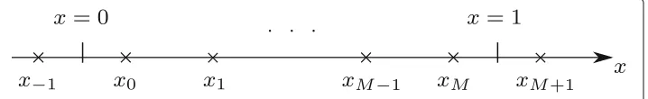
Let us first recall the Lax-Wendroff method [12]. Consider the advection equation
ut+aux=0, t>0, x∈[ 0, 1] , (6)
whereais a constant. The boundary condition remains to be discussed in Section6. We
approximate (6) by assuming that the solution is sufficiently regular, and take the Taylor series expansion at any point(x,t)to obtain,
u(x,t+t)=u(x,t)+t∂u
∂t(x,t)+
t2 2
∂2u
∂t2(x,t)+O
t3. (7)
A key step is thetemporal-spatial couplingtechnique by taking use of (6) to quantify the differentiation relation between the change rate ofuand the spatial variation,
∂u
∂t = −a
∂u
∂x,
∂2u ∂t2 =a
2∂2u
∂x2. (8)
Ignoring truncation errors of order more than three, the Lax-Wendroff scheme is derived as (cf. [12]),
un+j 1=unj −λ 2
unj+1−unj−1
+ λ2
2
unj+1−2unj +unj−1
, λ=at
x, (9) where central difference approximations are made to guarantee the spatial accuracy,unj represents the point valueuxj,tn
at the grid pointxj,tn
,xj =jx,tn=nt, with the
spatial and temporal incrementsxandt. The Taylor expansion process is the same as
that in the Cauchy-Kowaleveski approach (see [3]), and therefore (9) is regarded as the numerical realization of the CK approach. Note that this process determines the feature of this scheme, implying its application only in the range of hyperbolic problems (local behavior or finite propagation property). Any other extension needs serious and cautious treatments.
The Taylor expansion also relies on the smoothness of the solution. The successive differentiation (6) gives rise to the risk in the following sense.
(i) Once Eq.6admits discontinuities in the solution, the manipulation for (8) does not make any sense. This is the main reason that (9) produces oscillations near
discontinuities [12].
(ii) As this method is applied to highly nonlinear dynamical systems, this manipulation becomes horrible and hampers to develop higher order accurate schemes, due to the successive differentiations.
We will comment on this manipulation appropriately at later sections. Rather now, we reinspect (6) and (7) from another point of view (after ignoring high order truncation errors), actually in the finite volume framework,
u(x,t+t) =u(x,t)+t∂∂t u+ 2t∂∂ut
=u(x,t)−at∂∂x u+ 2t∂∂ut,
(10)
where the differentiation relation ∂∂t = −a∂∂x is applied. We immediately realize that for any(x,t)
u(x,t)+ t 2
∂u
∂t =u
x,t+t 2
as long as the solution is smooth in t (temporal direction or flow direction).
Viewing (10) in the finite volume framework, we obtain over the control volume
xj−1
2,xj+12
×[tn,tn+1),xj+1 2 =
1 2
xj+xj+1
,
u∗
j+1 2
:=uxj+1 2,tn
+ t
2 ∂∂ut
xj+1 2,tn
,
un+j 1=unj −λ
u∗j+1 2 −
u∗j−1 2
.
(12)
The prediction of the value u∗j+1 2
depends on the approximations to u
xj+1
2,tn
and
∂u
∂t
xj+1 2,tn
. This is achieved by theLax-Wendroff solver.
Lax-Wendroff solver.A Lax-Wendroff solver for(6)is the numerical algorithm approxi-mating the values
unj+1 2
:= lim
t→tn+0
uxj+1 2,t
, ∂u ∂t n j+1 2
:= lim
t→tn+0 ∂u
∂t
xj+1 2,t
(13)
for the given initial data at t=tnfor(6).
This pair of values actually provide all quite detailed information along the interface x=xj+1
2 of control volume and also the flux
1
t tn+1
tn au
xj+1
2,t
dt =au
xj+1 2,tn+
t
2
+Ot2
=a un j+1 2 + t 2 ∂u ∂t n j+1 2
+Ot2.
(14)
The two formulae (9) and (12) are equivalent for smooth flows. However, the new
formulation (12) is fundamentally different from (9) in the following sense.
(i) The formulae (12) is actually the finite volume formulation for (6). The formulation is more straightforward for fluid dynamical systems than other formulations because it is just the numerical version of balance laws and allows discontinuities as its solution.
(ii) The manipulation (11) is legal because the flow should be smooth in time (but not in space), unlike the difference approximation for LW approach.
(iii) The temporal-spatial coupling feature again plays an important role, e.g.,
∂u
∂t
xj+1 2,tn
= −a∂u
∂x
xj+1 2,tn
. (15)
This feature is crucial for a numerical scheme to preserve the fluid dynamical properties such as the Galilean invariance.
(iv) The successive differentiation (8) can be avoided, which is extremely important for nonlinear problems when discontinuities are involved because the manipulation (8) makes no sense both mathematically and physically.
For (6), we label “2” for the pairu,∂∂utin the Lax-Wendroff solver (13), which is the building block, as we see, in the Lax-Wendorff scheme. It is interesting to observe that
(13) can be approximated in an upwind or central way. The upwind approximation can
2.4 Lax-Wendroff flow solvers for nonlinear hyperbolic balance laws
We consider hyperbolic conservation laws
ut+f(u)x=0, (16)
where the vectoruis the conservative variable. The natural formulation of (16) is in the finite volume framework, the balance law over any intervalIj=
xj−1
2,xj+12
,
d
dtu¯j(t)= −1x
f
u
xj+1
2,t
−f
u
xj−1
2,t
,
¯
uj(t)= 1x
Iju(x,t)dx,
(17)
or the control volume
xj−1 2,xj+12
×(tn,tn+1),
¯
un+j 1= ¯unj − t x
fj+1
2 (tn;tn+1)−fj−12(tn;tn+1)
, (18)
with
¯ unj = 1
x
Ij
u(x,tn)dx, fj+1
2(tn;tn+1)=
1
t tn+1
tn
fuxj+1 2,t
dt. (19)
If one would prefer to other formulations, such as the discontinuous Galerkin method [2], the following statements still hold.
We shift(xj,tn)to (0, 0)due to the invariance of (16) with respect to the translation
of coordinates. In order to proceed in one of those frameworks, we have to solve (16)
approximately subject to the initial data
u(x, 0)=P±(x), for±x>0, (20)
whereP±(x)are smooth functions, typically polynomials, with a jump atx=0. The same as in the linear case (13), aLax-Wendroff flow solverfor such a problem is an algorithm approximating
u0:= lim
t→0+u(0,t),
∂
u ∂t
0 = lim
t→0+ ∂u
∂t(0,t). (21) In general, we consider hyperbolic balance laws in multi-dimensions,
ut+ ∇ ·F(u)=h, F=
fx,fy,fz
. (22)
wherehis the source term resulting from physics or geometry,x=(x,y,z)is the spatial coordinate. The initial data for (22) is set to be
u(x,y,z, 0)=P±(x,y,z), for±μ·x>0, (23)
whereμis the unit normal of a line or planeL : μ·x= 0 pointing from the negative
side to the positive side, corresponding to the outer normal of interfaces of computational volume. The Lax-Wendroff solver for (22) is to find the pair of values with the same form as in (21),
uL,0:= lim
t→0+u(L,t),
∂
u ∂t
L,0
:= lim
t→0+ ∂u
∂t(L,t), (24) where the limit is taken along the spatial-temporal interfaceL×(0,t).
We want to remark here that the pair uL,0,(∂u/∂t)L,0
2.5 Rough comments on the correlation between LW solver and temporal-spatial coupling
The instantaneous temporal derivatives in (21) and (24) can be roughly using the Lax-Wendroff approach
∂u
∂t = −∇ ·F(u)+h, (25)
and then−∇ ·F(u)andhare approximated using certain technologies such as WENO
etc. The same as in (15), the coherent relation of spatial and temporal variations is rooted in this formula.
The intuitive outcome of this coupling is the following.
(i) The multidimensional effect, in particular the transversal effect, is input into the flux directly. Thinking of a single advection problem
ut+aux+buy=0, (26)
wherea,bare constants. For an interface with the normal in thex-direction, the transversal effect, expressed in they-direction, is ignored for the standard Riemann solver. This is further verified for the wave system
pt+c0ux+c0vy=0, ut+c0px=0, vt+c0py=0, (27)
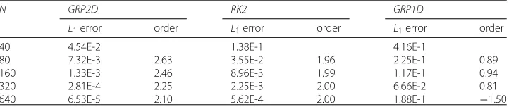
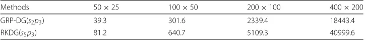
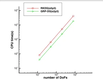
wherec0is a constant. In Table1, we use three methods to simulate the periodic
wave problem. It is observed that even with the same convergence rate, the RK method produces also ten times of errors than what the second order GRP does for which the transversal effect is included. The solution cannot even converge with the refinement of meshes if only normal flux is used but the transversal effect is not included. See [14].
(ii) The source effecthis also reflected through such a process. It is simple to see that
∂u
∂t = −
∂f(u)
∂x +h(u,x), (28) for hyperbolic balance law
∂u
∂t +
∂f(u)
∂x =h(u,x). (29) This input is essential and indispensable for the well-balancedness, as verified for the shallow water equations [15].
There are more fundamentals, such as the thermodynamical effect [16], resulting from the temporal-spatial coupling.
Table 1L1error and convergence order ofufor the periodic wave problem at final timet=2 with the methodsGRP2D,RK2andGRP1D
N GRP2D RK2 GRP1D
L1error order L1error order L1error order
40 4.54E-2 1.38E-1 4.16E-1
80 7.32E-3 2.63 3.55E-2 1.96 2.25E-1 0.89
160 1.33E-3 2.46 8.96E-3 1.99 1.17E-1 0.94
320 2.81E-4 2.25 2.25E-3 2.00 6.66E-2 0.81
2.6 22=4: Two-stage fourth order accurate schemes
In [4], the fourth order accurate method is developed for hyperbolic conservation laws. We start with the review of the dynamical system
d
dtw=L(w), (30)
whereL is a linear or nonlinear operator ofw. Then we have the following two-stage
algorithm for (30).
Stage 1. Define intermediate values
w∗=wn+ 12tL(wn)+ 18t2∂
∂tL(wn),
∂
∂tL(w∗)= ∂∂uL(w∗)L(w∗),
(31)
where the second equation follows from (30), using the chain rule.
Stage 2. Advance the solution using the formula
wn+1=wn+tLwn+1
6t
2
∂ ∂tL
wn+2∂
∂tL
w∗. (32)
This algorithm provides a fourth order accurate approximation tow. Originally, this
algo-rithm was proposed in [7, 17], and independently in [4] based on Lax-Wendroff flow
solvers. Along this direction, one can derive as high order accurate approximations as what he likes [7,18].
When applied to hyperbolic problems (16) and (22), one can formulate them in any
appropriate framework such as finite volume framework [4] or discontinuous Galerkin
(DG) framework [19]. Hence we assume that the computational domainis meshed as
= ∪j∈Jjand formulate the problem in the form
d
dtwj(t)=Lj(w), wj= 1
|j|
j
u(x,t)dx, w=wj;j∈J
. (33)
Thus, this problem boils down to the dynamical system in the form (30). Then we have a
two-stage fourth order time-stepping method, now symbolized as the “22=4” method.
The intuitive meaning is that we adopt the second order flow solvers as building blocks and use a two-stage time-stepping to achieve fourth order accurate numerical methods for hyperbolic problems or convection-dominated problems. We make a diagram in the following.
“4: A fourth order scheme = “2: Second order Lax-Wendroff type flow solvers
+ “2: A two-stage time stepping
Careful readers may observe the validity of (33) when the above two-stage algorithm
applies to the current case, which is why we have to develop the Lax-Wendroff type flow solvers based on hyperbolic balance laws rather than the formal partial differen-tial equations (Ben-Artzi, M, Li, J: On the consistency and convergence of finite volume approximations to hyperbolic balance laws, submitted). There are at least two points that
we should concern: (i) System(33)is index-dependent and therefore each equation for
fixed j is related to the neighboring equations; (ii) the continuity ofLjis crucial when
algorithm. Physically speaking, this regularity is natural by recalling the Lagrangian form of fluid dynamical systems [20]. Hence in the computation of instantaneous values (21) or (24), we must be aware of the regularity of the flux that will be further emphasized in the next section about the GRP solver.
3 The GRP solver: a discontinuous and nonlinear LW flow solver
As is well-known, and also pointed out in the last section, the standard Lax-Wendroff solver results in an algorithm that producing oscillatory solutions if discontinuities are present. The GRP solver, the abbreviation of the generalized Riemann problem (GRP) solver, can be regarded as the discontinuous and nonlinear version of the Lax-Wendroff solver. This solver was originally proposed in [21] for compressible fluid flows and related
problems. See [22] for the comprehensive summary of works before 2003. Later on a
direct Eulerian version of GRP solver was derived in [23] and further extended to gen-eral hyperbolic conservation laws [24,25]. The presentation below will follow the direct Eulerian GRP. The application to non-conservative systems is referred to [26].
3.1 1-D GRP solver
We first review one-dimensional GRP solver for hyperbolic balance laws
ut+f(u)x=h(x,u), (34)
subject to the initial data of form (20). An important prototype is the compressible Euler equations with cross section,
∂(A(x)ρ) ∂t +∂(
A(x)ρu) ∂x =0,
∂(A(x)ρu) ∂t + ∂(
A(x)ρu2)
∂x +A(x)
∂p
∂x =0,
∂(A(x)ρE)
∂t +
∂(A(x)u(ρE+p)) ∂x =0,
(35)
where the variablesρ,u,pandEare the density, velocity, pressure and the total specific energy. The total specific energy consists of two partsE = u22 +e,eis the internal spe-cific energy. The functionA(x)is the area of the duct. WhenA(x) ≡ 1, the system (35)
represents the planar compressible Euler equations. LetT be the temperature. Then the
entropyScan be defined, as usual, by Gibbs relation of thermodynamics,
TdS=de− p
ρ2dρ. (36)
The local sound speedcis defined as
c2= ∂p(ρ,S)
∂ρ . (37)
We will distinguish the linear (acoustic) and nonlinear GRP solvers. Both are related. However, as strong waves are involved, the nonlinear GRP solver becomes crucial. Details can be found first in [27] and later in [24,25] for general versions.
We denote
u=P−(0−0), ur=P+(0+0),
u=P−(0−0), ur=P+(0+0).
(I) Linear GRP solver.Linear hyperbolic equations describe the propagation of waves linearly. For the single linear case (6),
ut+aux=αu, (39)
with a damping constantα, we have obviously
u0=
a+ |a|
2 u+
a− |a| 2 ur,
∂
u
∂t
0
= −a+ |a|
2 u
−a− |2 a|ur+αu0. (40)
For the linear or semi-linear system case
ut+Aux=h(u,x), (41)
we need to diagonalize the system and pursue the characteristic decomposition. Denote by λ1,· · ·,λm the eigenvalues of A, = diag(λ1,· · ·,λm), and | | =
diag(|λ1|,· · ·,|λm|). Then we decomposeAasA = R R−1, and denote again|A| = R| |R−1. It turns out that the instantaneous values take
u0= A+|2A|u+A−|2A|ur,
∂u ∂t
0= − A+|A|
2 u− A−|A|
2 ur+h(u0, 0).
(42)
Therefore, the GRP solver for the linear system case is substantially the same as that for the single equation case.
(II) Acoustic Approximation
For nonlinear cases, ifu=ur, butu−ur =0, only linear waves emanate from the
singularity point(0, 0). Then we can linearize the system (34), at the valueu0=u=ur,
as
θt+A(u0)θx=h(x,u0), θ =u−u0, (43)
whereA(u0)is the Jacobianf(u0). Note that
∂u ∂t
0 =
∂θ ∂t
0
, and
yyyu
yx
0 =
∂θ ∂x
0
. (44)
Immediately we have
∂
u ∂t
0
= −A(u0)+ |A(u0)|
2 u
−
A(u0)− |A(u0)|
2 u
r+h(u0, 0). (45)
We can proceed to obtain any higher temporal derivatives(∂mu/∂tm)0, abbreviated as
ADER in [28]. However, in the framework of 22 = 4, we are satisfied with the first
order temporal variation in (45).
Asu−ur 1, weakly nonlinear waves emanate from(0, 0). Then we can carry out
the so-calledacoustic approximation.To be precise, we can use either exact or approxi-mate Riemann solvers to obtain the intermediate stateu0and linearize the system (34) to
be in the form (43) so that the temporal derivative(∂u/∂t)0is calculated as in (45). For the Euler Eq.35, the acoustic approximation is the following.
(i) Asu0−c0>0oru0+c0<0, the acoustic waves moves to one side of thet-axis.
(ii) Asu0−c0<0<u0+c0, thet-axis is located between two acoustic waves. Then
we have ∂u
∂t
0= − 1 2
(u0+c0)
u+ p
ρ0c0
+(u0−c0)
ur− pr
ρ0c0
,
∂p
∂t
0= −
ρ0c0 2
(u0+c0)
u+ ρp
0c0
−(u0−c0)
ur− pr
ρ0c0
−A(0)
A(0)ρ0c20u0.
(46)
The quantity(∂ρ/∂t)0is solved according to the direction of the contact discontinuity,
∂ρ
∂t
0 = 1
c20
∂
p
∂t
0 +u0
p−c20ρ (47)
ifu0=u=ur>0; and
∂ρ ∂t
0 = 1
c20
∂p
∂t
0 +u0
pr−c20ρr (48)
ifu0=u=ur<0.
For “cheap” engineering applications, one can use the local Riemann solutionu0 to
linearize the nonlinear system and obtain a “linear” system so that the above acoustic approximation strategy can be adopted.
(III) Nonlinear GRP solver
Asu−ur 1, nonlinear waves emanate from the singularity point(0, 0). The larger
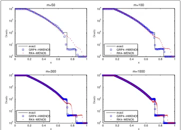
the difference betweenu andur is, the stronger the strength of the waves is. In Fig.1
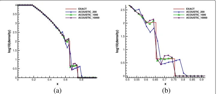
we use the acoustic GRP solver to simulate thebig density ratio problemand observe that the numerical solution has large disparity from the exact solution. In Fig.2, we use the nonlinear GRP solver that will be described below, and see that the numerical solution is improved prominently [16]. Hence it is essential to develop the nonlinear GRP solver as long as strong waves need resolving. We just illustrate the nonlinear GRP solver for Euler equations with cross section (35). For general hyperbolic balance laws, readers are referred to [24,25].
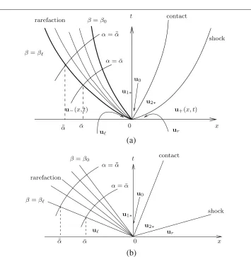
We just need to assume a typical case, as shown in Fig.3, that a rarefaction wave moves to the left, a shock moves to the right and a contact discontinuity lies in the middle. When
(a)
(b)
(a)
(b)
Fig. 2The GRP simulation (only 100 cells are shown).aGRP with relatively small number of grid points.
bZoomed solution
(a)
(b)
Fig. 3Typical wave pattern for the generalized Riemann problem.aWave pattern for the GRP. The initial datau(x, 0)=u+xuforx<0 andu(x, 0)=ur+urxforx>0.bWave pattern for the associated
the waves move to one side oft-axis, i.e.,u−c > 0 orur+cr < 0, it is treated as the
acoustic case that(∂u/∂t)0is obtained upwind. We rewrite (35) in terms of(ρ,u,S),
∂ρ ∂t +u
∂ρ ∂x+ρ∂
u
∂x = − A(x)
A(x)ρu,
∂u
∂t +u∂ u
∂x +
1
ρ∂∂px =0,
∂S
∂t +u∂∂Sx =0,
(49)
wherepis regarded as a function ofρandS. In terms ofρ,uandp, the third equation of (49) can be replaced by,
∂p
∂t +u
∂p
∂x +ρc
2∂u ∂x = −
A(x) A(x)ρc
2u. (50)
In order to resolve strong rarefaction waves, it is particularly essential to introduce the so-calledgeneralized Riemann invariants, as in [24],
φ=u−
ρ c(ω,S)
ω dω, ψ=u+
ρ c(ω,S)
ω dω. (51)
Together with the entropy variableS, system (35) becomes
⎧ ⎪ ⎪ ⎪ ⎪ ⎨ ⎪ ⎪ ⎪ ⎪ ⎩
∂φ
∂t +(u−c)∂φ∂x =B1,
∂ψ
∂t +(u+c)
∂ψ ∂x =B2,
∂S
∂t +u∂∂Sx =0.
(52)
whereB1 = T∂∂Sx + A
(x)
A(x)cu,B2 = T∂ S
∂x − A(x)
A(x)cu. Here it is easily seen that the variable
sectionA(x)acts on the dynamical behavior ofφandψ, and thus on that of(ρ,u,p). The severe change of entropy inevitably leads to the variation of other physical variables. The GRP solver that we will derive tells precisely how the entropy and the cross section affect the dynamics.
The most important ingredient is the application of nonlinear geometric optics for the local expanding of rarefaction waves using local characteristic coordinates(α,β), as shown in Fig.3. With that, we can obtain the instantaneous temporal derivatives∂S/∂t and∂ψ/∂tas (restricted to polytropic gases),
T∂∂St(0,β)= −(β+cθ)θ
2γ γ−1TS
, θ =c(0,β)/c, ∂ψ
∂t(0,β)=G1+ A(0)
2A(0)G2,
(53)
whereTS is defined through the Gibbs relation,
TS=e− p
ρ2
ρ
andG1,G2are given by,
G1= −β+ccθθ
γ+1
γ−1TS
+β+c2cθθ
3−γ
2(γ−1) 2γ
3γ−1TS−cψ
,
G2=β(β+cθ)−(β+2cθ)
uθ
3−γ
2(γ−1) +G2
,
G2=
⎧ ⎪ ⎪ ⎨ ⎪ ⎪ ⎩
−2(γ+1)cθ
(γ−1)(3γ−5)
1−θ25(γ−−3γ1)
− (γ+1)ψ
γ−3
1−θ2(γ−3−γ1)
, ifγ =3, 5/3,
2c(θ−1)−ψlnθ, ifγ =3,
2 [cθlnθ+ψ(1−θ)] , ifγ =5/3.
(55)
For general cases, please refer to [29].
Several remarks are in order about the role of entropy variation and the cross section on the dynamics.
(i) The source term reflecting geometric variation always plays an important role in the dynamics of flows. Inherently, the critical gas indices are clearly exhibited in (55), which cannot be illustrated in other flow solvers. This is just an evidence that only GRP solver can distinguish different gases.
(ii) The entropy change rate is essential and acts on other flow variables as its initial variation is severe. This tells why the GRP solver is indispensable when strong waves are simulated. As the involved waves are weak orT∂∂Sx is small,∂∂St is negligible and many approximations such as linearization are acceptable.
The shock is resolved by tracking its trajectory described by the Rankine-Hugoniot relation,
σ = ρu−ρu
ρ−ρ , u=u±(p;p,ρ), ρ=(p;p,ρ), (56)
where(ρ,u,p)and(ρ,u,p)are the states ahead and behind the shock, respectively, and
(p;p,ρ)=(p−p)
1−μ2
ρp+μ2p, (p;p,ρ)=ρ
p+μ2p p+μ2p, μ
2= γ −1
γ +1, (57)
for polytropic gases.
For the contact discontinuity x = x(t), we make use of the continuity property of
pressure and velocity on both sides of the trajectory,
u(x(t)−0,t)=u(x(t)+0,t), p(x(t)−0,t)=p(x(t)+0,t). (58)
Then the differentiation along the contact discontinuity gives Du
Dt(x(t)−0,t)= Du
Dt(x(t)+0,t), Dp
Dt(x(t)−0,t)= Dp
Dt(x(t)+0,t), (59) whereD/Dt=∂/∂t+u∂/∂xis the material derivative. This relation bridges the rarefac-tion wave and the shock, just like that for the Riemann solver. We just remind that the density and entropy undergo jump across this contact discontinuity.
Thus we come to the nonlinear GRP solver that are distinguished as nonsonic and sonic cases.
a∂∂ut0+b∂∂pt
0=d,
ar ∂u
∂t
0+br
∂ p
∂t
0=dr,
(60)
where a, b, dand ar, br, dr are specified below. Also the computation of(∂ρ/∂t)0are
computed by the following two cases.
(i) If u0 > 0, the contact discontinuity moves to the right and separates two states (ρ0,u0,p0),(ρ0r,u0,p0). The coefficients a, band dare given as,
(a,b,d)=(a˜,b˜,d˜). (61)
The coefficients ar, brand drare given by
ar= c 2 0
c2 0−u20
˜
ar
1− ρ0u20
ρ0rc20r
+ ˜br(ρ0r−ρ0)u0
,
br = c21 0−u20
˜
ar
− 1
ρ0 +
c2 0
ρ0rc20r
u0− ˜br
−ρ0r
ρ0u
2 0+c20
,
dr= ˜dr+ A
(0)
A(0) u
3 0 c2
0−u20
˜
ar
1− ρ0c20
ρ0rc20r
+ ˜br(ρ0r−ρ0)c20
.
(62)
The value(∂ρ/∂t)0is computed from the rarefaction side,
∂ρ
∂t
0 = 1
c20 ⎡ ⎣∂p
∂t
0
+(γ −1)ρ0u0
c0
c 1+μ2
μ2
TS ⎤
⎦, (63)
by using the state equation p=p(ρ,S).
(ii) If u0<0, the contact discontinuity moves to the left. The coefficients ar, brand drare
given as,
(ar,br,dr)=
˜
ar,b˜r,d˜r
. (64)
While the coefficients a, band dare computed by
a= c
2 0r
c20r−u20
˜
a
1− ρ0ru20
ρ0c20
+ ˜b(ρ0−ρ0r)u0
,
b= c2 1 0r−u20
˜
a
− 1
ρ0r +
c2 0r
ρ0c20
u0− ˜b
−ρ0
ρ0ru 2 0+c20r
,
d= ˜d+AA((00)) u30 c2
0r−u20
˜
a
1− ρ0rc20r
ρ0c2 0
+ ˜b(ρ0−ρ0r)c20r
.
(65)
The value(∂ρ/∂t)0is computed from the shock side,
gρR
∂ρ
∂t
0 +gpR
Dp Dt
0 +guR
Du Dt
0
where gρR, gpR, guRand frare constant, explicitly given in the following,
gRρ =u0−σ0, gpR= cσ20 0r −
u0H1, guR=ρ2∗(σ0−u0)·u0·H1,
fr= (σ0−ur)·H2·pr+(σ0−ur)·H3·ρr−ρr·
H2c2r+H3
·ur
−A(0)
A(0) ·
H2c2r+H3ρrur,
(67)
and H1, H2and H3are expressed by
H1= ρr(1−μ 4)p
r
(pr+μ2p0)2, H2=
ρr(μ4−1)p0
(pr+μ2p0)2, H3= p0+μ2pr
pr+μ2p0. (68)
The other coefficients
˜
a,b˜,d˜
and
˜
ar,b˜r,d˜r
are
˜
a(0,β)=1,
˜
b(0,β)= ρ(0,β)1c(0,β),
˜
d(β)= β+c2θc ·θ
3−γ
2(γ−1) 2γ
3γ−1TS−cψ
+ A(0) 2A(0)G2,
(69)
and
˜
ar=1− uσ20u0 0−c20r −
σ0ρ0rc20r
u2
0−c20r ·1
,
˜
br = ρ10ru2σ0 0−c20r −
1− σ0u0 u2
0−c20r
1,
˜
dr=LRp·pr+LRu·ur+LRρ·ρr+A
(0)
A(0)jr,
(70)
where we use notations
LRp= −ρ1
r +(σ0−ur)·2,
LRu=σ0−ur−ρr·c2r ·2−ρr·3,
LRρ=(σ0−ur)·3,
jr= −
2c20r+3ρrur+(1+1ρ0ru0)σ0c 2 0ru0 u2
0−c20r
;
σ0= ρ0ru0−ρrur
ρ0r−ρr , 1= 1
2
1−μ2
ρr(p0+μ2pr) ·
p0+(1+2μ2)pr
p0+μ2pr ,
2= −1 2
1−μ2
ρr(p0+μ2pr) ·
(2+μ2)p0+μ2pr
p0+μ2pr ,
3= −p0−pr 2ρr
1−μ2
ρr(p0+μ2pr).
(71)
Proposition 2(Sonic case). Assume that the t-axis is located inside the rarefaction wave associated with u−c. Then we have
∂u ∂t 0= 1 2 ˜
d+θ
2γ γ−1TS
+A
(0)
A(0)u20
, ∂ p ∂t 0=
ρ0c0 2
˜
d−θ
2γ γ−1TS
− A
(0)
A(0)u20
,
(72)
whered˜is given in(69), withθ = c0/c, and(u0,ρ0,c0)is the limiting value of(u,ρ,c)
The above formulae look complicated, but seem irreplaceable. We can go to [24] for technical derivation of them.
3.2 Temporal-spatial coupling and thermodynamical effect
Thermodynamics distinguishes compressible fluid flows from incompressible ones, and the Mach number can be regarded as a parameter of the compressibility. The entropy dissipation is a necessary condition guaranteeing the stability of numerical schemes. Let’s consider the compressible Euler equations with uniform cross section (A(x) ≡ constant in (35)). The entropy inequality says
(ρS)t+(ρuS)x≥0, inD. (73)
However, it is a well-known open problem whether this inequality is satisfied at dis-crete level, particularly for high order accurate schemes. There are two origins of disdis-crete errors: the data projection and the flux approximation. In a general setting of finite vol-ume framework, given the initial dataun(x)∈Pkatt =tn, we have to find the solution un+1(x)at next time levelt=tn+1, satisfying
xj+1 2 xj−1
2 ρ
S(un+1(x))dx ≥ xj+1
2 xj−1
2 ρ
S(un(x))dx
−t
(ρuS)approxj+1
2 −(ρ
uS)approxj−1 2
+Tol(x,t),
.
(74)
where(ρuS)approx
j+1 2
is the numerical entropy flux, andTol(x,t)is the entropy produc-tion that has the maximum tolerance of order three,Tol(x,t)= Ot3+x3. We comment on how to achieve this inequality at the discrete level in the following.
(i) The persistence spacePkoften consists of piecewise polynomials of degreek.
Given the initial dataun(x)∈Pk, we solve (35) and obtain the (analytic) entropy
solutionu(x,t)fortn<t<tn+1, satisfying
xj+1 2 xj−1
2 ρ
S(u(x,tn+1))dx≥
xj+1 2 xj−1
2 ρ
S(un(x))dx
− tn+1 tn ρuS
xj+1
2,t
dt−tn+1 tn ρuS
xj−1
2,t
dt.
(75)
(ii) The projection ofu(x,t)ontoPk(reconstruction procedure) is required to satisfy xj+1
2
xj−1 2
ρS(un+1(x))dx≥ xj+1
2
xj−1 2
ρS(u(x,tn+1))dx+Ox3. (76)
This is an extremely difficult step. For scalar conservation laws, there was a nice discussion on MUSCL-type linear reconstruction [30]. In general, the Jensen inequality tells that
ρS
¯ un+j 1
≥ 1
x xj+1
2 xj−1
2
ρS(x,tn+1)dx,
¯
un+j 1= 1x xj+1
2 xj−1 2
u(x,tn+1)dx.
(77)
(iii) Assume that (76) holds for certain data projection. As shown above, we approximate the interface value in the following way
u(xj+1 2,t)=u
n j+1
2 +
∂
u ∂t
n
j+1 2
(t−tn)+O((t−tn)2), tn<t<tn+1. (78)
In particular, we make use of the entropy information. It turns out that
(ρuS)approx
j+1 2
:=(ρuS)(xj+1
2,tn+12)=
1
t tn+1
tn
ρuS(xj+1
2,t)dt+O(t 2). (79)
Summarizing all together yields (74).
It is observed that the precise calculation of entropy in (53) is a direct way to achieve (79). Other ways may at most lead to
(ρuS)approxj+1 2
:=(ρuS)
xj+1 2,tn+12
= 1 t
tn+1
tn
ρuS(xj+1
2,t)dt+O
u2. (80)
The error ofOu2is not tolerated unless for scalar cases or smooth flows, since this type of errors violate the entropy inequality in the limit.
It is no doubt that the achievement of (79) is the outcome of the direct use of the entropy
equation in (49), which is actually the Lax-Wendroff procedure, a temporal-spatial
coupling procedure.
3.3 M-D GRP solver and transversal effects
When computing multidimensional (M-D) problems, M-D GRP solver is necessary to reflect the transversal effect, which is impossible using the exact or approximate normal Riemann solvers. We restrict to two-dimensional hyperbolic balance laws
ut+f(u)x+g(u)y=h(x,y,u), (81)
wherefandgare flux functions. 3-D GRP solver is straightforward. The initial data takes the form
u0(x,y)= ⎧ ⎨ ⎩
u−(x,y), x<0,
u+(x,y), x>0,
(82)
whereu±(x,y)are two polynomials of degreek. Thex-direction is the normal and the y-direction is the transversal. A particular case is
u0(x,y)= ⎧ ⎨ ⎩
u−+ ∇u0,−·x, x<0,
u++ ∇u0,+·x, x>0.
(83)
The M-D GRP solver can be classified asM-D linear GRP solver, acoustic GRP solver,
nonlinear normal GRP solver with transversal perturbation, and genuinely nonlinear M-D GRP solver.
(I) M-D linear GRP solver.We consider the linear case
ut+Aux+Buy=0, (84)
whereAandBare constant matrices, and both of them have their respective real
eigen-values and the complete sets of eigenvectors. We first assume that (84) is subject to the initial data (83). Note that∇usatisfies the same form of (84),
but subject to the initial data
∇u0(x,y)= ⎧ ⎨ ⎩
∇u0,−, x<0,
∇u0,+, x>0.
(86)
This boils down to the standard Riemann problem for∇u. Therefore, the gradient∇u
has an explicit expression,
∇u(x,y,t)=
L(x,t)
=1
∇v0,+r+ m
=L(x,t)+1
∇v0,−r, (87)
where the notationsL(x,t)is the maximum value ofsuch thatx−λt > 0,λis the eigenvalue ofAandris the associated eigenvector,vis so defined that
u= m
=1
vr, v=v1,· · ·,vm. (88)
See [31]. In particular, we have
∇u(0,y,t)= :λ<0
∇v0,+r+
:λ>0
∇v0,−r. (89)
Then we immediately obtain ∂u
∂t
0 :=limt→0+∂ u
∂t(0,y,t)
= −Alimt→0+ ∂∂ux(0,y,t)−Blimt→0+ ∂∂uy(0,y,t)
= −(A,B)· ∇u(0,y, 0+).
(90)
As far as the more general initial data (82) is concerned, the solutionuconsists of piece-wise polynomials of the same degree as the initial data since (84) is a linear system. Here we are satisfied with the second order GRP solver and solve (84) at any point(0,y0, 0)to
obtain
∂
u ∂t
0
= −(A,B)· ∇u0,y0, 0+
, (91)
where∇u0,y0, 0+
are calculated as the same procedure as above.
(II) M-D acoustic GRP solver.
For nonlinear cases (81), if the initial data (82) is continuous but discontinuous in its
derivatives, acoustic waves emanate from the interfacex = 0, just as one-dimensional
case. For this case, we might as well take the initial data (83) and assume thatu−=u+but
∇u0,−− ∇u0,+ =0. Then we linearize (81) around the stateu0=u−=u+to obtain θt+f(u0)θx+g(u0)θy=h(x,y,u0), θ =u−u0. (92)
Then we can exactly follow the linear case to calculate(∂u/∂t)0.
The acoustic approximation applies for the caseu−−u+ 1. We linearize (81)
around the intermediate stateu0resulting from the associated Riemann problem. Then
the linear GRP solver applies for this case.
(III) M-D genuinely nonlinear GRP solver with transversal description.
Asu−−u+ 1, we have to deal with genuinely nonlinear GRP. Thinking of the
initial value problem for (81) subject to the initial data (83), the solution is the envelope
Riemann solution is known. For example, at two points(0,y1, 0)and(0,y2, 0), we solve
the Riemann problem locally for the normal conservation law, respectively,
ut+f(u)x=0, (93)
and obtain the local intermediate valuesu(0,y1, 0+)andu(0,y2, 0+). Then for any point (0,y, 0),y1<y<y2, we can approximate∂∂uy(0,y, 0+). Particularly, we approximate
uy
0,y0, 0+
= u
0,y1, 0+
−u0,y2, 0+
y1−y2 +O
(y1−y2)2
. (94)
Then we regard the transversal termg(u)yandh(x,y,u)as a perturbation locally, and
solve the following problem,
ut+f(u)x= −g(u)y+h(x,y,u)=:d(x,y,u,uy). (95)
This boils down to the one-dimensional planar problem locally, for which the GRP solver was proposed in [24]. Detailed and complete M-D GRP solver is proposed in [32].
3.4 Transversal effects for genuinely M-D schemes
For multidimensional (M-D) problems, the balance law can be always written in the form,
d dt
u(x,t)dx= −
∂f(u)·ndL, (96)
whereis the control volume,∂is the boundary andnis the outer unit normal. We
ignore the external force just for the clarity of presentation.
Thanks to the Galilean invariance, we always assume that(1, 0)(the directionx-axis) is the normal direction, and(0, 1)(the direction ofy-axis) is the transversal direction. The standard Riemann solver just reflects the normal effect. In contrast, the LW procedure can describe the transversal effect precisely. Consider a linear advection problem
ut+aux+buy=0. (97)
Then we use the temporal-spatial coupling property to obtain
∂
u
∂t
∂= −a
∂
u
∂x
∂−b
∂
u
∂y
∂, (98)
where (∂∂ux)∂ and (∂∂uy)∂ can be obtained by solving the associated Riemann prob-lem. Also as remarked in Section2for the linear wave system, the transversal effect is substantial even though the convergence rate is formally the same.
4 The kinetic LW flow solver
The fluid dynamics can be described in various viewpoints, such as the kinetic descrip-tion. The governing equation is the Boltzmann-type equation
ft+ξ · ∇xf =
1
B(f,f), (99)
wheref = f(t,x,ξ)is the density distribution,ξ is the velocity of molecules (particle), andB(f,f)is the collision term,is the Knusner number. Ideally, for a given initial dis-tribution, we solve (99) to obtain the solutionf
t,xj+1
2,ξ
and define the numerical flux
fj+1
2(tn;tn+1)=
1
t tn+1
tn
whereψ=(1,ξ,ξ2)is the invariant, and the average of macroscopic variables is
un+j 1= 1 x
xj+1 2
xj−1 2
3ψf(tn+1,x,ξ)dξdx. (101)
In general, it is difficult to solve the Eq.99analytically. To understand the relation of macroscopic equations (Euler and Navier-Stokes equations) and the kinetic equation, we first take theso-called railroad methodin [33] as an example to illustrate how to devise kinetic schemes.
4.1 Railroad method
Consider the linear advection equation
ut+aux=0, u(x, 0)=u0(x). (102)
Introduce a distribution functionf(t,x,ξ)and define the macroscopic variableu(x,t)as
a moment off,
u(x,t)=
∞
−∞f(t,x,ξ)dξ. (103)
If we choosef to take the form,
f(t,x,ξ)= u√(x,t)
π exp −(ξ−a)2
, (104)
thenf(t,x,ξ)satisfies
ft+ξfx =Q[f] := (ξ−
a)
√π exp −(ξ−a)2∂u
∂x, (105)
subject to initial data
f(0,x,ξ)= u√0(x)
π exp −(ξ−a)2
. (106)
The initial value problem (102) and the problem (103)-(106) are equivalent: If one solution is known, then the other is defined. We write the solution of (105)-(106) as
f(t,x,ξ)=f(0,x−tξ,ξ)+
t
0
Q[f](τ,x−(t−τ)ξ),τ,ξ)dτ. (107)
Then the solutionu(x,t)is given as
u(x,t)=
∞
−∞f(0,x−tξ,ξ)dξ+
∞
−∞
t
0
Q[f](τ,x−(t−τ)ξ),τ,ξ)dτdξ. (108)
Note that the LW approach for (107) yields
f(t,x,ξ)=f(0,x,ξ)+tξ ∂
∂xf(0,x,ξ)+tQ[f](0,x,ξ)+O
t2. (109)
Therefore we have
u(x,t)=
∞
−∞(f(0,x,ξ)+tξ
∂
∂xf(0,x,ξ)+tQ[f](0,x,ξ))dξ+O
t2, (110)
which yields a second order approximation to the exact solutionu(x,t). The numerical solution is
uj(t)=uj(0)−
t
x
Fj+1 2 −Fj−12
where
uj(t)= 1x xj+1
2 xj−1
2
∞
−∞f(t,x,ξ)dξdx,
Fj+1 2 =
t
0
∞
−∞ξf(t,xj+1
2,ξ)dξdt.
We assume the initial data for (102) is piecewise smooth with possible discontinuity at x= xj+1
2. Correspondingly, the initial data (106) for (105) consists of two parts. It turns
out that the numerical fluxFj+1
2 in (111) becomes
Fj+1 2 =F
+ j+1
2 +
Fj+−1 2
, (112)
whereF±
j+1 2
consist of three parts, respectively,
Fj+±1 2 =
t
0
±ξ>0ξf
τ,xj+1 2,ξ
dξdτ =tG±j+1 2 −
t2 2
Hj+±1
2 −
Kj+±1 2
,
Gj+±1 2 =
±ξ>0ξf
0,xj+1
2 ∓0,ξ
dξ,
Hj+±1 2 =
±ξ>0ξ2∂∂xf
0,xj+1 2 ∓0,ξ
dξ,
Kj+±1 2 =
±ξ>0ξQ[f]
0,xj+1
2 ∓0,ξ
dξ.
(113)
As the solution is smooth, the scheme (111) becomes the LW approach immediately. See
[33] for details.
4.2 The LW type solver for gas kinetic schemes
Let’s now work on a simplified model, the Bhatnagar-Gross-Krook (BGK) model [34],
ft+ξfx=
g−f
, (114)
whereis the collision time, andgis the equilibrium state, approached byf asgoes to zero,
g= ρ m
m
2πkT 3
2
e−(m/2kT)ξ2, (115)
wheremandkare constant,ρandT are density and temperature, respectively. Indeed,
all macroscopic variablesρ,uandEare defined as
(ρ,u,E)(x,t)=
3
1,ξ,ξ2f(t,x,ξ)dξ. (116)
The validity of BGK-model is clearly explained in [34].
Starting with (114), Xu and his collaborators successfully developed gas kinetic scheme (GKS) solver [35–39]. A key ingredient is that the explicit solution formula for (114) is used for the numerical flux approximation,
f(t,xj+1 2,ξ)=
1
t
0
g(t,x,ξ)e−(t−t)/dt+e−t/f0
xj+1
2 −ξt,ξ
, (117)
subject to the initial dataf0(x,ξ), where x = xj+1
2 −ξ(t− t
). Here just the case of
one-dimension is described. The full information contained in (117) provides “exact”
expression of flux across the interfacex = xj+1
2, which is of course consistent with the
LW flow solver. We can go to [38] for comprehensive description of the GKS solver.