ENG470 Engineering Thesis
1
ENG470 Engineering Thesis S2 2015
Investigation into the Functionality and Operation of
the Spi-Sun Simulator
A report submitted to the School of Engineering and Energy, Murdoch University in partial fulfilment of the requirements for the degree of Bachelor of Engineering (Honours)
Student: Abdulrahman Al-Dajani Supervisor: Dr. David Parlevliet
Due Date:16/02/2016
ENG470 Engineering Thesis
2
Abstract
For various reasons, both economic and ecological, the production of PV cells has been
expanding during the last decade. Inherently the need for better quality control, rating and
qualifying methodology has also become equally increasing.
As PV modules would differ in both material and quality, building testing equipment that can be
used to rate as well as to improve the light-energy conversion qualities have become an essential
part of the PV industry.
Solar simulators used for indoor testing of PV modules measure the performance characteristics
under non-standard conditions to adjust and reproduce the results based on the standard
conditions defined by a number of international testing codes.
In addition to the calibration required which is characteristic for all measuring apparatus, a closer
understanding of the technology behind the simulator, operation and the form of produced result
and their significance is essential for progressive improvement of the quality rating as well as for
the further development PV technology.
A set of IV (Current-Voltage) measurements have been performed on a PV module of certain
parameters and results were obtained and analysed to interpret the significance of the effects of
testing as well as to explore PV module conditions. The tests were conducted using a Spi-Sun
5600 SLP simulator.
The results reflected the effects of light intensity, shading and temperature and concluded with
providing a set of recommendations for mitigating their negative effects and identifying favourable
conditions for maximizing the PV output.
The thesis endeavours at bringing together relevant required technical material for understanding
the background of the technicalities involved and provides an introduction in PV testing for future
ENG470 Engineering Thesis
3
Disclaimer
I declare the following to be my own work, unless otherwise referenced, as defined by the University’s policy on plagiarism.
ENG470 Engineering Thesis
4
Acknowledgments
I would like to acknowledge the efforts of Dr. David Parlevliet throughout the development of this
thesis. His constant supervision, guidance, support and encouragement have been vital in
ENG470 Engineering Thesis
5
Contents
Abstract ... 2
Disclaimer ... 3
Acknowledgments ... 4
1. Introduction ... 7
2. Thesis Overview ... 8
3. Solar Energy and Photovoltaics ... 10
4. Theory of Operation ... 12
4.1 Solar Simulator ... 12
4.1.1 Light Sources ... 13
4.1.2 Power Supplies ... 14
4.1.3 Optics ... 14
5. Performance Parameters ... 15
6. Literature Review ... 16
6.1 Spi-Sun Specifications and Operation Theory ... 16
6.2 Theory of Operation ... 19
6.3 Spi-Sun and Other Solar Simulators ... 21
6.3.1 Standards ... 21
7. Design considerations ... 23
7.1 Other Applications of Simulators ... 26
8. Introduction and significance of IV Curves ... 29
9. Modules Under Test ... 33
9.1 190W Module ... 33
9.2 230W Reference Module ... 33
10. Methodology ... 35
10.1 Familiarisation Tests ... 35
10.2 Calibration Tests ... 40
10.2.1 Test Setup ... 41
10.3 Light Intensity Tests ... 41
10.4 Temperature Correction Tests ... 42
11. Results ... 44
11.1 Familiarisation Tests ... 44
11.2 Calibration Tests ... 48
11.3 Light Intensity Tests ... 49
11.4 Temperature Correction Tests ... 51
12. Discussion ... 54
12.1 Familiarisation Tests ... 54
12.1.1 Normal Test Run ... 54
12.1.2 IEC vs ASTM Standards ... 54
12.1.3 Shaded Cells ... 55
12.1.4 Solutions for dealing with Shade ... 56
12.2 Calibration Tests ... 58
12.3 Light Intensity Tests ... 60
12.4 Temperature Correction Tests ... 61
13. Undergraduate Study Guide and Lab Exercises ... 63
13.1 Lab 1 – Safe Operation of Simulator ... 64
13.2 Lab 2 – Familiarisation with the Simulator ... 65
13.3 Lab 3 – More Specific Functions ... 65
Lab Guide Example ... 67
14. Scope of Future Work ... 69
15. Conclusion ... 70
16. References ... 72
Appendices ... 77
Appendix A ... 77
6
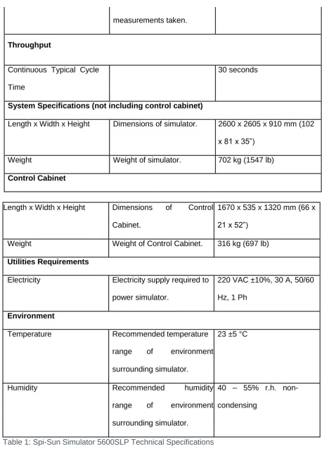
Table 1: Spi-sun Simulator 5600SLP Technical Specifications……….……16
Table 2: Table of abbreviations used in the discussion of I-V curves………...30
Table 3: 190W Module Specifications………...…33
Table 4: 230W Reference Module Specifications………..………...33
Figure 1: The I-V and P-V curves of a photovoltaic device………….. ... 30
Figure 2: The Fill Factor ... 31
Figure 3: Several Categories of losses that can reduce PV array output ... 32
Figure 4: Test Device Parameters Window……….36
Figure 5: Test Configuration Window……….37
Figure 6: Lamp Calibration Window ... 40
Figure 7: Test Information Window ... 42
Figure 8: IV and Power Curves - Normal Run... 44
Figure 9: IEC vs ASTM - Normal Run IV Curves ... 46
Figure 10: IEC vs ASTM - Normal Run Power Curve ... 46
Figure 11: IV and Power Curves of Module with Shaded Cells. ... 47
Figure 12: Calibration Data Drift - Maximum Power between readings ... 48
Figure 13: IV Curves for different light intensities (200 W/m2 - 1000 W/m2) ... 49
Figure 14: Plot of Maximum power against Light Intensities ... 50
Figure 15: Plots of Isc and Voc against Light Intensities ... 50
Figure 16: Power Curves for different Light Intensities ... 51
Figure 17: MPP vs Temperature. ... 51
Figure 18: Voltage variation vs Temperature. ... 52
Figure 19: Current vs Temperature………..…53
ENG470 Engineering Thesis
7
1. Introduction
The performance of a solar simulator used for testing and rating PV modules can be affected by a number of factors, for example “simulator bulb type, age, current and alignment affect the spatial
uniformity, temporal stability and spectral irradiance” (Emery 1986).
This project aims to explore and investigate the functionality and operation of a new PV module
performance test simulator by conducting a series of I-V measurements under controlled
temperature and spectral conditions.
To achieve this objective, tests are developed, automated, reviewed and analysed, for the
Spi-Sun 5600 SLP Simulator. Calibration procedures are carried out and maintenance guidelines are
reviewed.
Analysis of test results and associated uncertainty analyses are also presented.
The Spi-Sun 5600SLP Simulator, manufactured by Spire Corporation of Massachusetts, is a
photovoltaic module measurement apparatus that can perform a range of tests under controlled
temperature and spectral conditions. This modern and complex machine establishes a new
standard in module measurements, as it can perform measurements to a high level of accuracy
and precision, thus providing efficient and reliable data acquisition.
The simulator’s ability to apply different spectral conditions enables it to perform measurements
at different wavelengths and light intensities. Its low profile design and small footprint enables it to
easily integrate into any type of environment. It can also support testing of PV modules of different
ENG470 Engineering Thesis
8
2. Thesis Overview
The aims and objectives of the thesis include the following:
i. Gain insight into solar energy as a source of renewable energy.
ii. Understand the solar simulator concept with its related components and types.
iii. Develop methodologies and Techniques in PV Power Measurements
a. Gaining a broader insight and looks into the different techniques used to perform PV
power measurements. This will include looking into different simulator types available
in the industry and the range of applications they are used for.
b. Comparing and contrasting different types of simulators.
c. Specifically looking into the Spi-Sun Simulator and how it performs measurements on
PV modules.
iv. Calibration of the Simulator
a. Learn about the system’s calibration procedures and parameters and how they
influence performing measurements.
b. From a technical point of view, performing calibration measurements regularly on a
calibration module in order to investigate how far calibrated data drifts from one
reading to another.
v. Operability and Functionality Study of the Spi-Sun 5600 SLP Simulator
a. Looking into the different features of the simulator to clarify functions and the
significance of related variables such as spectral, spatial and temporal variables,
which will help establish any limitations the Spi-Sun simulator might have as well as
advantages over other types of simulators.
b. Exploring the simulator’s performance by looking into how it provides standard test
conditions at different temperatures. Some experimental results will be described in
this report.
ENG470 Engineering Thesis
9
a. Exploring the underlying variables that contribute to the simulator’s accuracy and
repeatability of the measurements it takes.
vii. Undergraduate Study Guides/Laboratory Sheets
a. Developing a set of study guides for undergraduate students that offer insight into how
the simulator works. Exposing students to the simulator and having them perform a set of tasks and related analysis will aid in understanding the simulator’s different
operation parameters.
The thesis will conclude by confirming that these objectives have been achieved, and will provide
ENG470 Engineering Thesis
10
3. Solar Energy and Photovoltaics
Modern times have emphasised the use of sustainable renewable energy instead of fossil fuels
for the many advantages the former has over the latter. But what makes a source of energy a
renewable one? In general terms, renewable energy “comes from natural sources that are
constantly and sustainably replenished” (Nrdc.org 2015). The aim of renewable energy is to
provide and promote better life quality on all fronts and reduce the reliance of communities on
fossil fuels and finite sources.
Solar energy is one type of renewable source of energy that utilises sunlight. There are many
benefits in using solar energy, that including:
Clean source of energy with greatly reduced emissions.
More affordable than other types of renewable sources.
Does not require an extensive amount of maintenance.
There is no noise pollution associated with electricity generation.
Solar energy technologies are divided into two main types:
(1) Photovoltaics, where photovoltaic cells convert sunlight into electricity. Photovoltaic cells form modules and arrays that are installed on “rooftops, integrated into building designs and vehicles, or scaled up to megawatt scale power plants” (Australian Renewable Energy Agency 2013).
(2) Solar Thermal technology: these are systems that convert sunlight into thermal energy. They
are commonly used in many applications including space and water heating, refrigeration cycling
and electricity generation using steam turbines. Such systems are typically integrated into large
scale generators producing tens to hundreds of megawatts (Australian Renewable Energy Agency
2013).
Solar technologies have had significant impact on the way Australia utilises solar energy. This is
supported by the following facts:
Australia has the highest average of solar radiation available per square meter.
ENG470 Engineering Thesis
11
The continent’s electricity demand can easily be met as there is more than enough
roof space to be utilised by solar panels.
Economically wise, solar energy systems have reduced the size of electricity bills.
Government offers grants and incentives for any grid connected system, thus
attracting more consumers to switch to solar energy (Solar Content 2015).
With such demand for solar energy and photovoltaics, an evolving, growing energy market has
developed to supply different consumer types with required services. With that increase of growth,
solar panel and system prices have decreased. They are now estimated to be $1000 per kilowatt
for Solar Panels and around $2000 - $3000 per kilowatt for PV systems (including of solar panels,
DC to AC inverter, mounting cable and other electrical accessories) (Tressider 2013). As stated
earlier, electricity generated by photovoltaics has become a competitive and cheaper alternative
ENG470 Engineering Thesis
12
4. Theory of Operation
4.1 Solar Simulator
Before going in depth on how the Spi-Sun performs its functions and operations and what makes
it unique in comparison to other types of simulators, a brief description on what components
makes up a solar simulator in a general sense and on what a solar simulator particularly aims to
do shall be presented.
According to Wang, a solar simulator is an important tool in establishing a common basis of
comparing between different types of solar cells, as well as providing data for designing
large scale systems (Wang 2014). Consequently, solar simulators play a vital role in solar
PV cell testing and development.
According to ASTM (American Society for Testing and Materials), which is an organizational body
that develops and publishes technical standards that serve a wide range of products in different industries, such as metals, petroleum, construction, etc. (Astm.org 2016). “A solar simulator (also
artificial sun) is a device that provides illumination approximating natural sunlight. The purpose of
the solar simulator is to provide a controllable indoor test facility under laboratory conditions, used for the testing of solar cells, sun screen, plastics, and other materials and devices” (ASTM 2015).
Generally, solar simulators are composed of a number of major components. The ASTM suggests and states that “a solar simulator usually consists of three major components: (1) light source(s)
and (2) associated power supply; (3) any optics and filters required to modify the output beam to meet the classification requirements” (Solar Simulators - A Guide 2015).
The following sections will provide more details on the types of simulator components that are
ENG470 Engineering Thesis
13
4.1.1
Light Sources
For light sources, there are a number of lamp types that can be found in solar simulators. The following bullet points briefly describe some of the commonly used sources:
Xenon Arc lamps: Xenon lamps were widely used in the 1960s. Being an artificial source,
they provide a very close spectral match to the solar spectrum. This source delivers good uniformity and output stability that many photovoltaic cell manufacturers can apply and utilise in testing. Despite its positives, this source is considered expensive compared to other arc sources; this is due to an ever increasing demand for a limited global supply of Xenon. (Solar Simulators - A Guide 2015)
Metal Halide Arc Lamps (HMI): Commonly used in film and television lighting. They are a
good alternative to Xenon lamps as they are “more stable, provide better temporal stability,
easier to maintain and cheaper” (Solar Simulators - A Guide 2015). Metal Halide lamps
offer reduced spectral perturbations in infrared than Xenon lamps, meaning they are more
suitable for use in advanced solar simulators.
Light Emitting Diodes (LED): Recent and rapid technological advancements gave rise to LEDs
that are used in a lot of industries. The most unique features of LEDs are their low consumption of energy and a longer lifetime than most lamp types. Despite these features, LEDs are limited in their spectral wavelength as they are only available in discrete wavelengths. A cluster of LEDs operating at different wavelengths would be required to produce a full spectrum; although the cluster will still only produce a crude approximate of the solar spectra. This limitation also means that LEDs are not useful in “advanced, multi junction devices that have a spectral range past 1000nm” (Solar Simulators - A Guide 2015).
Quartz Tungsten Halogen Lamps (QTH): These offer a relatively assured black-body
match in the infrared part of the solar spectrum but poor match on the visible end. They
offer good output stability and do not produce strong UV light emissions (Newport.com
2015). Tungsten lamps are more commonly used in advanced simulators utilising multiple
ENG470 Engineering Thesis
14
4.1.2 Power Supplies
Power supplies will differ from one source to another depending on the power requirements of
the simulator. Complex solar simulator configurations that utilise energy consuming arcs will
require complex power supplies that are able to supply a high voltage to initiate a light arc.
Systems that use lower energy consuming LEDs or Tungsten lamps are more likely to make
use of simpler DC sources (Solar Simulators - A Guide 2015).
4.1.3 Optics
The optical setup of a solar simulator is influenced by some important factors, such as “the type
and number of light sources used, area illumination generated, and spectral output generated etc” (Solar Simulators - A Guide 2015).
Generally, most solar simulator manufacturers will incorporate a parabolic reflector, a mixing
mirror and an infrared clipping filter. Xenon sourced systems could incorporate a 90 degree, down
facing mirror. Most concerns associated with the optics of a system lie in the ease of
ENG470 Engineering Thesis
15
5. Performance Parameters
The IEC 60904-9 Edition2 and ASTM E927-10 are two examples of common specification
standards that solar simulators adapt for photovoltaic testing. Classification of solar simulators is
based on the three following parameters:
i. Spectral match
The spectral match of a simulator indicates how much of the spectrum of sunlight can filter through a certain thickness of the earth’s atmosphere. The Spi-sun simulator meets both IEC
and ASTM standards of AM 1.5. This means that the spectrum of sunlight has been filtered to
pass through 1.5 thicknesses of atmosphere. The previous spectral match value of AM 1.5
however corresponds to the condition of a module facing the sun directly on a clear, sunny day
at noon and is 60 degrees above the horizon. The filter is used to provide coverage for a certain
wavelength range depending on spectra.
ii. Spatial uniformity (expressed by degree of non-uniformity)
Uniformity of irradiance of the simulator beam over the test area. (Solar Simulators - A Guide
2015)
iii. Temporal Instability
Temporal instability is a characteristic of time where it measures the stability of the beam of
light over a specific time interval, 1s as per ASTM standards E927. This instability is measured and reported over a period of 100 ms, 1 minute and 1 hour. The sun’s radiation is stable over
time, international standards classified different simulators based on their temporal stability
ENG470 Engineering Thesis
16
6. Literature Review
This following section will provide some background literature to explain several aspects of the
thesis including:
Looking into the technical specifications of the Spi-Sun simulator and the theory behind
its operation.
Reviewing other solar simulator systems developed or available on the market.
How outputs of different systems are analysed, such as using IV curves or other
methods.
Standard test procedures and why they are used.
Some of the applications for the different simulators.
Information on the precision of each of the simulators introduced.
6.1 Spi-Sun Specifications and Operation Theory
This section will start off by outlining some of the technical specifications of the Spi-Sun simulator. These specifications were extracted from the simulator’s operation manual and will take the form
of a table with brief descriptions defining each variable.
The technical specifications enable later make comparisons between the Spi-Sun simulator and
other simulators.
Variable Description Value
Maximum Module Length 2000mm
Maximum Module Width 1370mm
Light Source
Number of Lamps Number of lamps embedded 2
in simulator that produce the
ENG470 Engineering Thesis
17
Lamp Type Type of lamp used to Single long pulse filtered
undertake tests. xenon tube
Pulse Duration The duration of one pulse 20 – 120 ms at 1000 W/m2
(flash) of light. This can be
adjusted to accommodate
different test scenarios.
Spectrum Spectrum range of ≤ ± 12.5%, AM 1.5 (Class
Simulator. A+)
Irradiance Temporal Stability A measure of irradiance over ≤ 0.2% at 1000 W/m2 (Class
a specified period of time. A+)
Irradiance Spatial Uniformity A measure of irradiance over ± 1% (Class A+)
a specified test area.
Lamp Life Number of lamp flashes 100000 Flashes
before it is recommended to
be replaced.
Measurement Range and Performance
Range of Light Intensity Light intensity range that can 200 – 1100 W/m2
be tested through simulator.
Measurement Duration Time it takes to take < 1 second
measurement.
Power/Module (max) Max module power simulator 600 W
can test.
Voltage Ranges 5 ranges (2.5, 10, 25, 100,
250 V full-scale)
Current Ranges 4 ranges (3, 6, 12, 25 A full-
scale)
I/V Resolutions 0.003%
ENG470 Engineering Thesis 18
measurements taken.
Throughput
Continuous Typical Cycle 30 seconds
Time
System Specifications (not including control cabinet)
Length x Width x Height Dimensions of simulator. 2600 x 2605 x 910 mm (102
x 81 x 35”)
Weight Weight of simulator. 702 kg (1547 lb)
Control Cabinet
Length x Width x Height Dimensions of Control 1670 x 535 x 1320 mm (66 x
Cabinet. 21 x 52”)
Weight Weight of Control Cabinet. 316 kg (697 lb)
Utilities Requirements
Electricity Electricity supply required to 220 VAC ±10%, 30 A, 50/60
power simulator. Hz, 1 Ph
Environment
Temperature Recommended temperature 23 ±5 °C
range of environment
surrounding simulator.
Humidity Recommended humidity 40 – 55% r.h. non-
range of environment condensing
surrounding simulator.
ENG470 Engineering Thesis
19
6.2 Theory of Operation
This section outlines the methodology the Spi-Sun simulator follows in performing its tests and
explains why it does so. This section will provide further verification to earlier sections that include
the components of a solar simulator as well as further explanation into some of the variables in
the table of specifications given above.
The Spi-Sun simulator is built and developed according to both IEC 60904-9 (Photovoltaic devices
– Part 9: Solar simulator performance requirements) and ASTM E927 (Standard Specification for
Solar Simulation for Terrestrial Photovoltaic Testing) standards. The simulator offers Class A
requirements for spectral match, temporal stability, and spatial uniformity as shown in the table.
Testing of photovoltaic devices is carried out under certain reference conditions of irradiation
exposure and air mass of less than 2.5. Due to the weather effects over the clarity of the sky,
varying air mass and temperature, varying solar exposure, unless a solar tracking system is
used, outdoor testing would require faster IV readers to minimize errors due to changing ambient
irradiance and therefore be more difficult to conduct. Consequently indoor testing provides a
controlled testing environment under stable conditions (TamizhMani et al. 2015).
As for most solar simulators, the Spi-Sun simulator is also comprised of three major components:
Light sources and associated power supplies.
Optics and filters, where they are selected to meet standard requirements.
Controls to operate the simulator, adjust irradiance, and record and display data.
Temporal stability, as defined earlier in section 5, page 15.
The temporal drift is reduced with the help of the silicon monitor cells attached onto the simulator.
Coupled to the electronic circuitry of the simulator, the cells monitor illumination intensities and manage pulse consistency, therefore, keeping the simulator’s temporal stability in check.
Since the data acquisition system may be affected by temporal instability, it is included in IEC
ENG470 Engineering Thesis
20 Simulator™ 5600SLP system records the values of irradiance, voltage, and current
simultaneously.
The spectral match: The simulator produces the light spectrum matching that of the standard
solar spectrum as defined by both IEC and ASTM AM 1.5 which relates to the spectrum of sunlight
that can filter through 1.5 thicknesses of atmosphere.
A calibrated spectrometer is used for simulator spectral irradiance measurements. The spectral
irradiance data is integrated over the wavelength intervals as defined by both (IEC and ASTM)
standards to determine the total irradiance. The resulting percentages, of total irradiance across
the standard wavelength ranges are compared with the percentages required by AM 1.5 Global
Spectrum. The irradiance deviations and the irradiance classification to IEC 60904-9 is
ENG470 Engineering Thesis
21
6.3 Spi-Sun and Other Solar Simulators
The following section explores some of the other solar simulator systems within the same AAA
classification which use different light sources and or optics, in as much detail as available
information allows, compares their attributes with the Spi-Sun simulator.
6.3.1 Standards
Standards have been developed to maintain “quantitative” consistency among different performance
criteria for photovoltaic cells and modules produced by manufacturers around the globe. The criteria includes energy conversion efficiency, quantum efficiency (ratio of number of collected carriers to incident photons) (PVEducation.org 2016a), and current-voltage characteristics. With many organisational bodies developing different standards, the primary standards organization that details solar simulator performance requirements, specifications, and test protocols is the International Electro-technical Commission (IEC; www.iec.ch). Other standards bodies includethe American
Society for Testing and Materials (ASTM; www.astm.org) and the Japanese Standards
Association (JSA; www.jsa.or.jp).
The three standards documents—IEC 60904-9 ed2.0, ASTM E927-10, and JIS C 8912—classify solar simulators with a three-digit “ClassXYZ” designation, where
X defines the spectral match (the ratio of the actual percentage of total irradiance to the required
percentage specified for each wavelength range). Spectral matching is specified by the percentage of total solar irradiance from a simulator that “must fall within each 100 nm wavelength
interval between 300 nm and 1100 nm. The previous stated range best simulates the spectral
output of the sun and was ideally selected to cover the absorption region of the early
single-crystal photovoltaic cells.
Y defines the spatial non-uniformity of the irradiance.
ENG470 Engineering Thesis
22 A solar simulator classified as ABB means that “it meets Class A spectral match, Class B spatial
non-uniformity, and Class B temporal instability specifications” (Gail Overton 2015).
Solar-cell and module manufacturers are required by ASTM and IEC standards to test using a
minimum Class BBB and Class ABC solar simulator, however, manufacturers using a Class AAA solar simulator— would benefit from the higher degree of matching the Standards criteria in
optimizing their manufacturing process as cells and module pricing is based on simulator data
and therefore using higher classification simulators that have very low error in simulation results
would prove beneficial.. Higher than Class AAA simulators would be required for special
ENG470 Engineering Thesis
23
7. Design considerations
Solar simulators are manufactured in different shapes and configurations. They differ in the
type of light source, System Optics, Controls and Working Area:-
i. Simulator Light Source
a. Xenon Light Source
The bright white light is produced by passing an electric arc through a bulb filled with xenon gas.
The light produced closely imitates the natural sun light.
Xenon Light sources can be categorized with respect to their construction and to their operation.
Construction wise Xenon lights can be of a short arc or a long arc lamp made so by manipulating
the arc producing portion of the lamp.
Operation wise Xenon lights can either be of the continuous light type (short arc and long arc
produce continuous type) or can be of a flash/pulsed type.
The continuous type uses two electrodes for producing the arc whereas the pulsed type contains
a third electrode that acts as a high voltage trigger to ionize the gas and a capacitor connected
to the two main electrodes to discharge through the ionized gas causing the flash. Flash/pulsed
types are also used for photographic applications and some other scientific applications
as well (Loflin 2016).
Simulators using pulsed xenon light have the drawback of short exposure time which makes them
limited to PV cells having an electrochemical response time within its pulse duration which is
unsuitable for testing longer response time such as thin film PV cells (Loflin 2016).
Spi-sun, however, uses single long pulse xenon light with adjustable pulse duration of 20 -120
ms. As such Spi-Sun combines the benefit of the relatively shorter exposure time along with the
consequential decrease in thermal stress on the tested cell and the adjustable pulse time to be
ENG470 Engineering Thesis
24 Other simulators such as Oriel Sol3A (Newport 2009) and Solar Light LS1000 (SolarLight 2016)
use continuous xenon short arc light with varying exposure timing using shutters which does not
share the response time limitations due to the larger adjustment of the shutter timing available
and a minimum exposure time of around 200ms and can therefore be used to test thin-film PV
technologies that cannot be otherwise characterized using pulsed sources.
The lifetime of continuous light is expressed in hours whereas pulsed type lifetime is expressed
in the total number of flashes.
Depending on the number of starts and end-of-life criteria, a 1.6 kW lamp with a 300 × 300 mm
illumination area has a lifetime of about 2,000 hours.
Testing using continuous light source, though increases the temperature of the tested PV cell,
can identify hot spots in solar cells (zones that heat disproportionately across the cell or module),
pulsed-source simulators however (such as Spi-Sun and IWASAKI (Eye.co.jp 2016)) minimize
cell/module thermal stress. However, according to a survey made by experts at PHOTON
International Magazine for single crystal or multi-crystalline cells, regardless of the thickness of
the cell there was no significant influence on the rate of the observed heat build-up effect when
cell was under the light for up to 500ms. A typical test takes about 120 ms. Thus the perceived
disadvantage of a SS system is not real (Gail Overton 2015).
b. LED-based Simulators
This light source is made up of a number of Light Emitting Diodes (or LED(s)) selected and
individually controllable to produce irradiance values distributed over wavelengths between
300nm and 1100nm thus simulating the AM1.5 spectrum complying with a Class A spectral
match. . Simulators using LED light source have longer exposure duration which are offset by
lower light wattage.
As an example, Newport Oriel VeraSol-2 Class AAA LED Solar Simulator independently “drives
multiple LEDs at 19 individual wavelengths spaced over the spectrum from 400 nm to 1100 nm
ENG470 Engineering Thesis
25
ii. Optics
Solar simulators have certain components in common such as the light source, reflectors and
controls. Some simulators such as the Newport Sol3A (Newport 2009) and Abet Sun3000 (ABET
Technologies 2015) using continuous Xenon Arc light utilize a shutter with an adjustable exposure
time which can be operated either automatically or manually. Spi-Sun does not use a shutter as
the light source is a long pulse with variable illumination timing, hence taking the role of the shutter.
Whereas both Spi-Sun and Sol3A (Newport 2009) use filters, WACOM WSLED models which use
LED as the light source achieves the solar matching by varying the individual illumination of the
LED group of lights and therefore does not use a spectral filter. Abet deliver one sun irradiances
over the lamp lifetime and limit UV exposure by utilizing an N-BK7condenser lens.
(Wacom-ele.co.jp 2015)
iii. Controls
The main purpose of the controls is to modify the testing environment to simulate external such as
variations in external environment solar exposure due to various weather conditions and to keep
temperature under control to minimise measurement errors.
The Spi Sun simulator uses a set of capacitors to control the energy and timing of the light pulse.
The Spi sun also includes a temperature controlled fixture on which the PV cell is placed. Also two
monitor cells, coupled to the electronic circuitry, monitor illumination intensity and manage pulse
consistency. The measured temperature of the module during testing enables temperature
compensation of the I-V data.(Spi-Sun 5600 SLP operation manual).
Solar simulators such as Newport Sol3A, using continuous light control light exposure using the
special design shutter along with a partial sun attenuator and controls the exposure duration.
ENG470 Engineering Thesis
26
iv. Working Area
Working area of solar simulators determines the maximum size of the PV cell under testing and
are comparable to the overall dimensions of the solar simulators and vary between as small as
50mmx50mm (Sun2000) or as large as 2000mmx1370mm (Spi-Sun) Oriel Sol3A (Newport 2009)
and Solar Light simulators have a relatively small working area (up to 203mm x 203mm and up to
152mmx152mm respectively) with varying light power and working distances.
In comparison the Spi-Sun simulators has a large working area of 2000mm x 1370mm, which
allows testing of larger PV modules at a fixed working distance and lamp size hence reducing the
number of physical simulator variables which improves the degree of measurement certainties
since variable working distances can affect irradiance uniformity, each model (working area) has
a specific working distance range.
Spi-Sun has an advantage over other types of testing PV modules in various array arrangements
due to its large working area.
7.1 Other Applications of Simulators
Some simulators, such as Newport Oriel Sol-UV simulators, provide other applications beside solar simulation, such as dermatological applications in scientific research to investigate and verify sun protection products for the skin; Commercially, Oriel UV solar simulators have been used by skin product manufacturers to verify their products' and make sure they comply with health agency standards including the FDA (The United States Food and Drug Administration). By complying to these standards, Newport have been able to develop unique light intensity and exposure controllers that are used to research skin products. Newport states, “By using our 68951 Exposure/Intensity Controller for
timed exposures or dose controlled exposures for in-vitro testing of samples or in-vivo testing of
volunteers, skin care product manufacturers are able to quickly determine the effectiveness of their
ENG470 Engineering Thesis
27 Other applications of solar and light simulators include being used as testing equipment for coating
and paint products, paper and labels, optical components, plastic and rubber. Solar simulators
can also be used for research purposes, such as in studying degradation and weathering, stability
of photos, agricultural use in exploring plant growth, packaging effectiveness, textile studies, and
transmission studies (Globalspec.com 2015).
Other available configurations and their applications also include:-
i. Solar simulator systems can take the shape of solar chambers. These solar chambers
consist of a power supply that powers the simulator system, a light source to provide light
flashing and testing conditions, and an enclosure that enables an operator to safely
function the simulator and system and protect him/her from any radiation that may emit
during and after testing (Globalspec.com 2015).
ii. Some simulator configurations utilise Flood lamps as their light source. Flood lamps
provide a wide beam of light. Systems using flood lamps can be operated as independent,
stand-alone systems or be part of a larger photovoltaic system and arrays
(Globalspec.com 2015).
iii. Systems can also be configured to use focused lamps. Focused lamps can be though as
opposites to flood lamps as they provide a narrow beam of light. Such systems can also
be operated as stand-alone system or part of a larger system (Globalspec.com 2015).
iv. With the many advancements in photovoltaic technology, some simulators and light
sources have become portable and handheld. This has increased the practicality of using
light sources in conditions and areas where the transportation of larger systems and light
sources is unrealisable. Such devices are suitable for repairing and testing in field,
laboratory, and plant floor applications (Globalspec.com 2015).
v. Spot or wand systems are light sources that provide a small spot and direct beam of light.
Such systems are vastly used in medical areas, precisely for dermatological applications
(Globalspec.com 2015).
vi. Lastly, wall and ceiling mounted systems also consist of a power supply and a light source.
ENG470 Engineering Thesis
28 to a wall or ceiling. Such systems can be used an air disinfectant where light sterilizes the
ENG470 Engineering Thesis
29
8. Introduction and significance of IV Curves
An IV (Current-Voltage) curve analysis defines the capability of a photovoltaic string of modules
or system to convert energy and produce power at existing conditions of light intensity and
temperature. Theoretically, an IV curve represents the current and voltage combinations at
which the photovoltaic system or string of modules operates. Determining the operability of the
system is dependent on the factors or light intensity and temperature being constant. Figures 1
and 2 below demonstrate a typical I-V curve. The figures also demonstrate the PV
(Power-Voltage) curve which is computed from the IV curve and the key points on these curves
(Solmetric 2011).
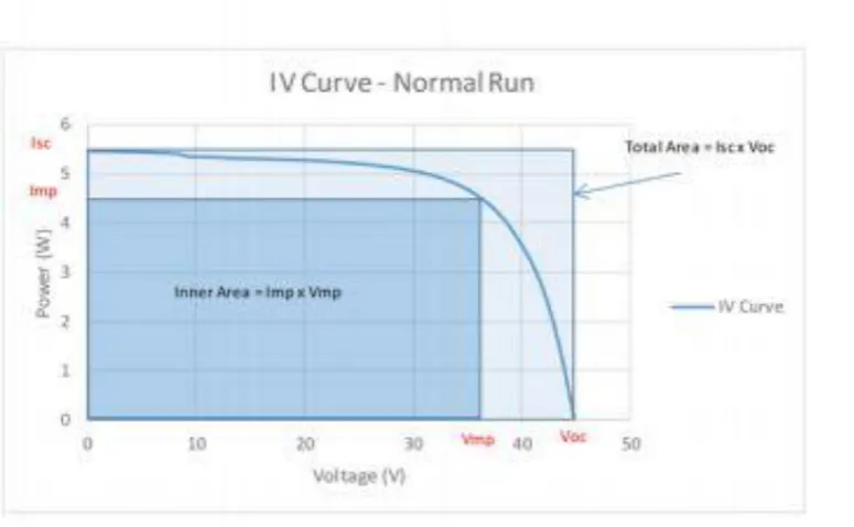
From figure 1, the span taken up by the IV curve ranges from the short circuit current (Isc) which
starts at the origin of the voltage axis - zero volts, to zero amps current at the open circuit voltage (Voc). The ‘knee’ of an IV curve indicates its maximum power point (Imp, Vmp) and is the point
where the array generates the maximum amount of power or electricity. In most advanced photovoltaic systems, an inverter in an operating photovoltaic system monitors and “tracks” the
system’s power outputs and always seeks the maximum power point so that maximum power
and electricity is yielded from the system (Solmetric 2011).
In more scientific terms, for voltages that are below the voltage at the maximum power point (Vmp), electricity generated is not dependant on the final voltage output. However, near the knee of the IV curve, this behaviour changes and the following is noticed:
An increase in voltage means a larger percentage of electrical charges come together and
ENG470 Engineering Thesis
30 Figure 1: The I-V and P-V curves of a photovoltaic device. The P-V curve is calculated from the measured I-V curve (Recreated from Solmetric 2011).
Please note the abbreviations listed in Table 2, below. They will be used throughout this
document.
Abbreviation Definition
Isc Short circuit current
Imp Max power current
Vmp Max power voltage
Voc Open circuit voltage
Vx Voc/2
Ix Current at Vx
Vxx Voltage midway between Vmp and Voc
Ixx Current at Vxx
FF Fill Factor = (Imp*Vmp)/(Isc*Voc)
Table 2: Table of abbreviation used in the discussion of I-V curves. (Solmetric 2011) Isc
ENG470 Engineering Thesis
31 The Fill factor (FF) of a photovoltaic system is one of the most important factors and performance indicators on which a system’s analysis is performed. The fill factor can be defined by the ratio of
two areas outlined under an IV curve. As shown in figure 2, the areas include the inner area determined by the maximum power point where Imp is multiplied by Vmp. The second “total” area
is defined by the short circuit current Isc multiplied by the open circuit voltage Voc. The ratio of
the (Imp x Vmp)/(Isc x Voc) indicates the value of fill factor. An ideal fill factor would be 1, this is not possible however as it is not physically possible to produce a “rectangular” IV curve response
where the maximum power point would coincide with Isc and Voc (Solmetric 2011).
The Fill Factor’s importance lies in its indication to how efficient an operating module or system
can be. The higher the Fill Factor, the more efficient the module is and thus the more power it is
expected to generate. The opposite is also true as a lower Fill factor entails a less efficient module
or system operation (Solmetric 2011).
Figure 2: The Fill Factor, defined as the gray area divided by the cross-hatched area, or (Imp x Vmp)/(Isc x Voc), represents the square-ness of the I-V curve. (Recreated from Solmetric 2011) Two photovoltaic modules of same model and type would have similar Fill factors under identical
conditions. However, different module technologies and design entitle different magnitudes of
fill factors. For instance, amorphous silicon modules would usually have lower fill factors, thus
ENG470 Engineering Thesis
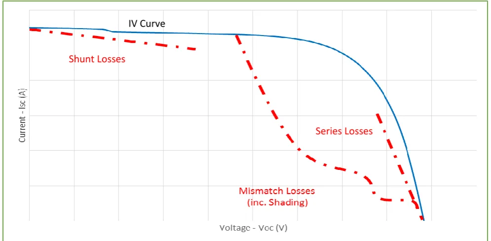
32 IV curves can also provide indications of any impairments that reduce the Fill factor. Figure 3
below shows some of the effects of shunt resistance losses, series resistance losses, and
mismatch losses (including shading parts of a module) where each loss contributes differently
to the shape of the IV curve. Uniform soiling is another impairment that may affect IV curves
and is defined by the less light reaching cells of a module. Soiling effects are observed by a
height reduction of the IV curve (Solmetric 2011).
Figure 3: Several categories of losses that can reduce PV array output. The I-V curve provides important troubleshooting clues (Recreated from Solmetric 2011).
Shunt Losses
ENG470 Engineering Thesis
33
9. Modules Under Test
This section will provide the specifications of the modules that were used in the various tests
performed throughout the development of this thesis. It will also state what module was used
for each test.
9.1 190W Module
The 190W module was used for the familiarisation, light intensity and temperature
correction tests. Its specifications are as follows:
Values at STC
Maximum Power Pmax 190 W
Voltage at Pmax Vmp 37.85 V
Current at Pmax Imp 5.02 A
Open Circuit Voltage Voc 46.55 V
Short Circuit Current Isc 5.37 A
Power Tolerance ±3%
Current Rating 10 A
Table 3: 190W Module Specifications
It is important to note that the above module is defective, as it contains some broken cells that
are visible. Therefore, outputs will vary. This is observed in the results as maximum power was
only 169 W.
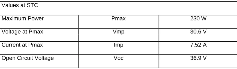
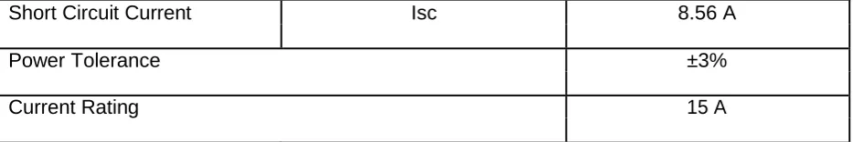
9.2 230W Reference Module
The 230W reference module was used in the calibration tests. Its specifications are as follows: Values at STC
Maximum Power Pmax 230 W
Voltage at Pmax Vmp 30.6 V
Current at Pmax Imp 7.52 A
Open Circuit Voltage Voc 36.9 V
ENG470 Engineering Thesis
34
Short Circuit Current Isc 8.56 A
Power Tolerance ±3%
Current Rating 15 A
ENG470 Engineering Thesis
35
10. Methodology
This section presents the methods and procedures applied to fulfil the thesis tasks. It provides
clarification on how some of the research material was introduced and how experiment-related
data was collected and analysed. This section will also assist in developing future thesis that may
include broader, more in depth aspects.
Firstly, an outline will be given of the steps taken to perform the various tests. These will take the
form of paragraphs detailing instructions taken and will also include some screenshots of the system’s interface showing what configuration of parameters would be assigned for each test.
10.1 Familiarisation Tests
To become familiarised with the simulator and its interface, a couple of basic tests were
performed. These tests gave an idea of what was measured and how it was measured.
The first test involved producing an IV curve and seeing what different variables the system
presented.
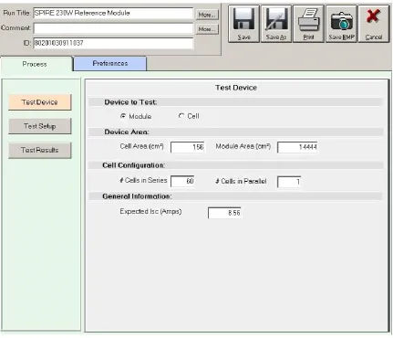
Before running the test, the parameters of the module under test were introduced onto the simulator’s setup. This was done by generating a new parameter setup file under the process tab
where some of the device under test’s characteristics are entered.
This incorporates the following as shown in the screenshot below:
Type of device tested: Whether a whole module or a specific cell is tested.
Device area: Inputting the module and cell area, this is to provide more accurate
measurements of efficiency.
Cell configuration: The number of cells in series and in parallel.
General information: The expected short circuit current is entered and is obtained from
ENG470 Engineering Thesis
36 Figure 4: Test Device Parameters Window
After the parameters are entered, they are saved and the module is tested.
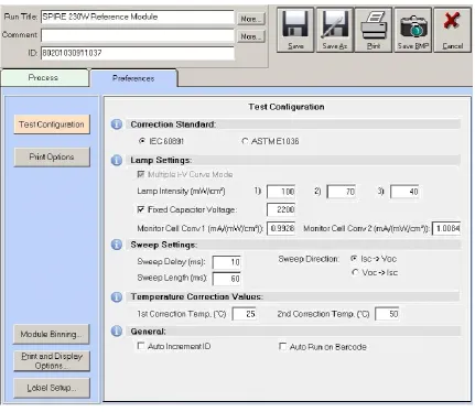
The second test was a simple one as it looked into what the differences were in setting up the
temperature correction factors per IEC and ASTM standards. To setup for a test, the parameters
window is opened and in the Test Configuration under the Preferences tab, a selection is made
as to what correction standard one wants to follow. The screenshot below shows the Test
ENG470 Engineering Thesis
37 Figure 5: Test Configuration Window
Further explanation of the test configuration’s window parameters are outlined as follows:
Correction Standard: Choosing between IEC 60891 and ASTM E1036 will result in
different settings for correcting an IV curve. The IEC 60891 standard utilises three
lamp intensities during a flash to produce IV curves. On the other hand, the ASTM
standard only uses single intensity during a flash. (Refer to page 79 of Operation
Manual).
Lamp Settings: Under the lamp settings, the Multiple IV Curve Mode allows for the
option to produce multiple IV curves with different lamp intensities. Lamp Intensity
allows for what light intensity is used. If the Multiple IV Curve Mode is enabled, then
ENG470 Engineering Thesis
38
Fixed Capacitor Voltage: If this is selected, the capacitor voltage can be set at a
fixed value. This can be left untouched and the simulator will calculate a suitable
value.
Monitor Cell Conv: This value is used to display the lamp irradiance, and is usually
set up during the light calibration procedure.
Sweep Settings: Under the Sweep Settings, the Sweep Delay accounts for the time
it takes between flashing and sampling IV data. Sweep length is how long the
sampling of IV data takes. Lastly, Sweep Direction offers the option of having the
data sampled from Isc to Voc or vice versa during testing.
Temperature Correction Values: 1st Correction Temperature is the primary
temperature correction value applied to readings and is usually set to 25°C as per
standard test conditions. The 2nd Correction Temperature value offers an
alternative temperature correction value if found needed.
That being said, visually there is no variation in the IV curves produced when either standard is
chosen; this statement will be proved through the curves presented in the Results chapter.
Each standard uses specific units that are determined by each standard’s different coefficients.
The following briefly describes the coefficients involved for each standard. Conversions from and
to each standard and examples, are provided in Appendix A.
The ASTM E1036 standard uses the unit of %/°C (Percentage per Degree Celsius). The
coefficients used to establish the unit are:
α (Alpha): The temperature coefficient for current.
β (Beta): The temperature coefficient for voltage.
δ (Delta): The intensity coefficient. Default value is set to zero.
PMax: Temperature coefficient used to adjust for PMax. Default value is set to zero.
The IEC 60891 standard uses the units of mV/°C volt per Degrees Celsius) or mA/°C
ENG470 Engineering Thesis
39 α (Alpha): The temperature coefficient for current.
β (Beta): The temperature coefficient for voltage.
K: Curve correction factor. Default value is set to zero.
The third and final familiarisation test involved observing the effect of shaded cells and how this
is reflected in the IV Curve it produces. This was done by shading part of the module under test
with a thick layer of paper. The test parameters and configurations applied were as for the previous
ENG470 Engineering Thesis
40
10.2 Calibration Tests
The calibration tests were performed by exposing a calibration, reference module to the simulator’s
flashes. Readings were taken at different times throughout the project. Analysis of the readings provided clearer insight on how often the simulator’s lamps needed to be calibrated.
Before delving into how I approached taking the measurements, it is useful to note what variables
can be calibrated and how.
The user can set up the simulator to calibrate either the lamp intensity by itself, or calibrate both
lamp intensity and Pmax, where Pmax is the maximum power output of the module.
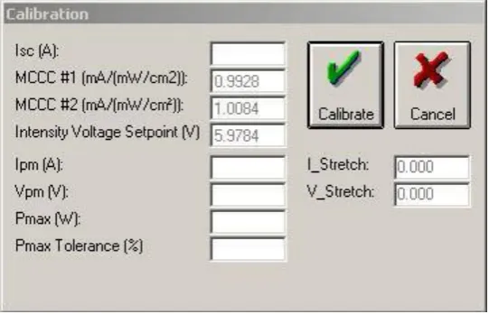
The Lamp Calibration Window shown below can be accessed by clicking Calibrate Lamps
under the Configure menu tab.
Figure 6: Lamp Calibration Window
Calibrating the Lamps would only require inputting the expected short circuit current, which is given in the calibration module’s label into the Isc (A) field. After the Isc is entered, clicking the
Calibrate button will simply perform the calibration procedure.
Calibrating both Lamp intensity and Pmax will require entering all values of short circuit current Isc,
maximum power current Imp and the maximum power voltage Vmp. From these values, the
simulator produces three IV curves where the first and second involve measuring current and
voltage data. The third IV curve is the lamp calibration curve and it is used to average Imp and
ENG470 Engineering Thesis
41
10.2.1 Test Setup
To set up the calibration test, it was decided that readings of the Calibration Module would be
taken on separate days. From the readings, current and voltage values were obtained and IV
curves were generated to give a visual interpretation of what was going on. From the current and
voltage values, the power was calculated for each point and a Power curve was added to the initial
IV curve. From the power values, the maximum power values were pulled out, which gave the
Maximum Power Point of the module.
Having followed the same steps for all calibration data, it was decided to use the Maximum Power Point as the primary feature to explore and analyse the drift between calibration readings.
The outcomes and analysis are presented in the following Results and Discussions Sections.
10.3 Light Intensity Tests
The following set of tests involved exposing the test module to a range of different light intensities.
The range of intensities used was 200 W/m2 to 1000 W/m2.
Setting up for this test was simple and straightforward. Most parameters associated to this test
remained unchanged and only the light intensity was varied. The light intensity can be changed in
ENG470 Engineering Thesis
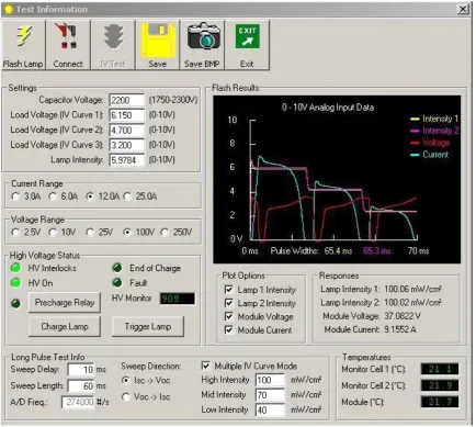
42 Figure 7: Test Information Window
After the intensity is changed, the information is saved and the module is tested.
The significance of using different light intensities in testing will be explained in the Discussions
section. The Discussions section will also introduce some information about the low light
performance of a module and in particular what effects this has on the series and shunt
resistances.
10.4 Temperature Correction Tests
The temperature correction test formed a fairly major part of this thesis from a technical point of view. It explored how the simulator applied temperature correction factors to standardise readings taken to
ENG470 Engineering Thesis
43 setting up an air conditioning unit to its lowest temperature set point a day earlier before running
the tests.
The day of the test would include taking regular readings of the module under testing while increasing the room’s temperature. The time between each reading would not be a significant
factor as the expectation is that the simulator will always apply the 25 degree correction factor no
matter the small changes in temperature. The range of temperatures the simulator was exposed
to was 17.8 to 29.7 degrees Celsius.
The test involved taking 33 test points between 9:10 am and 1:36 pm on Friday the 11th of
September. A full list of tests and their associated times is presented in the Appendix B
Taking readings was fairly straight forward and simple to perform. The module was flashed with
a light intensity of 1000 W/m2 as per standard test conditions as well.
From the IV curves produced, the power was calculated by multiplying the current and voltage,
similar to what was done with the calibration tests. From the list of power values, the maximum
power point was picked out and chosen to be the factor on which the analysis is performed on.
A graph of the trend obtained from the readings is presented in the Results section. Analysis and
further commentary on what the trend means and why it is so will be justified in the Discussions
ENG470 Engineering Thesis
44
11. Results
The following section is dedicated to providing results of the various tests undertaken through the
development of this thesis. The results are outlined in conjunction with the way the Methodology
section has been set up.
The results will briefly discuss what the presented graphs signify and some further commentary is
given on any trends that may have developed. Only key results are discussed in this section, and
graphs and plots presented summarize the findings.
11.1 Familiarisation Tests
The first test was a simple, normal run of the simulator that did not involve any manipulation of
configuration and test settings. It aimed at getting familiarised with the graphical interface of the simulator’s system and the common characteristics of the produced plots.
Figure 8: IV and Power Curves - Normal Run
The curves of current (I) versus Voltage (V) and Power versus voltage that were plotted for the
test run are illustrated in Figure 8.
ENG470 Engineering Thesis
45 The second familiarisation tests looked at what differences would be observed if the test was
configured to run per IEC and ASTM Standards. (Differences introduced in page 48 of Chapter
12.1.2)
Data points for each standard’s test run were plotted on the same graph so it is easier to observe
the difference. IV curves were plotted on one graph and Power curves were plotted on another to
ENG470 Engineering Thesis
46
IEC vs ASTM - Normal Run
C
u
rr
en
t
(A)
6
5
4
3
2
1
0
0 5 10 15 20 25 30 35 40 45 50
Voltage (V)
IEC ASTM
Figure 9: IEC vs ASTM - Normal Run IV Curves
Figure 10: IEC vs ASTM - Normal Run Power Curve
From both IV and Power curves produced in testing for both standards it is clear that the only
slight variation lies in the descending part of the curve and consequently the final value of voltage
(VOC) obtained from the readings. However, this is not a significant variation as it is not expected
ENG470 Engineering Thesis
47
The third and final familiarisation test involved running the simulator’s flash onto a module with
shaded cells.
Figure 11: IV and Power Curves of Module with Shaded Cells.
From the plot above, it can be observed how significantly a partially shaded module affects the power output of the module. From the module’s rated output of approximately 170W, the shaded
cells take the maximum power output down to about 98W. That’s an approximate 47% loss in
output power.
This also highlights the current limiting effect of partially shaded cells as indicated by the “kink” on
the graph at about 1 amps and 30 volts.
This effect can also be called “current mismatch” and is defined by the different current outputs of
each cell of that module. As cells of a module are connected in series, they must all have the
same amount of current running through. Realistically, what happens for shaded cells is that the
module settles on the output of its lowest performing cell, which would also be the cell that is more
heavily shaded than others. This results in the overall reduction in power output of the string
containing the shaded cells (Sargosis.com 2016).
The use of Bypass diodes can prove handy in avoiding the above repercussions of shaded cells.
ENG470 Engineering Thesis
48
11.2 Calibration Tests
Calibration tests were done to provide an idea of how often and when calibration procedures need to be performed on the simulator’s lamps. With the use of a reference module, current and voltage
characteristics are obtained and used to calculate the maximum power point. Ultimately, it was
decided that the variation of maximum power from one reading to another would be the
determining factor in analysing the drift between each.
The following plot shows the maximum power point and variation between each test.
Figure 12: Calibration Data Drift - Maximum Power between readings
The STDEV function in excel was used to calculate the standard deviation between each reading
and was about 1.065. From first view, this value represents a variation that is very small and can be overlooked in some applications. From the plot it is clearly observed that the “significant”
variation occurs between the readings taken on the 9th of September and 22nd of October. This is
due to the fact that there was a month and a half difference between these readings, but that also
gives rise to the suspicion that test configuration and setup data might not have been consistent
when these readings took place. Furthermore, readings from second to fifth test are much more
closely aligned as they were taken closer together and thus explains that it would be more
accurate to rely on the readings taken between the 22nd of October until the 9th of November.
ENG470 Engineering Thesis
49
11.3 Light Intensity Tests
This test has been set to explore the behaviour of a module when tested under a range of light
intensities.
Figure 13: IV Curves for different light intensities (200 W/m2 - 1000 W/m2)
From figure 13, an IV curve plot for the module under test at different light intensities is produced.
It is clear to deduce that as the intensity of the light increases, the current drawn from the module
increases along with an increased open circuit voltage VOC. With the higher currents being drawn
by higher light intensities, this would imply that higher power outputs are generated. This is also
ENG470 Engineering Thesis
50 Figure 14: Plot of Maximum power against Light intensities (200 W/m2 - 1000 W/m2)
The plot above shows the maximum power outputs for each of the light intensities tested. Along
with the IV curves, this plot clearly indicates the presence of an almost perfect linear relationship
between power and light intensity where more light intensity will result in larger power outputs
and vice versa.
Figure 15: Plots of Short circuit current Isc and Open circuit voltage Voc against light intensities.
The above plots of the short circuit current Isc and open circuit voltage Voc demonstrates that
both variables have a directly proportional relationship with light intensity. Short circuit current is
ENG470 Engineering Thesis
51 Figure 16: Power Curves for different light intensities (200 W/m2 - 1000 W/m2)
11.4 Temperature Correction Tests
As stated earlier, the temperature correction test was performed to demonstrate how the simulator
records measurements and adjust these readings to conform to standard test conditions of 1000
W/m2 and 25 degrees Celsius. A plot was produced that shows the maximum power point of the
module against the different temperatures the test runs were exposed to.
Figure 17: MPP vs Temperature
It is clearly seen that a trend has developed where the amount of power has decreased as the
ENG470 Engineering Thesis
52 drop from about 169 W to 158 W signifies about a 7% drop in power. That is quite a high
percentage considering the expectation that readings would be more closely consistent and to
some extent equal.
This decreasing trend is also reflected in the current behaviour with the varying temperatures as
shown below.
Figure 18: Voltage variation vs Temperature.
Figure 18 shows the plot of the open circuit voltage against temperature during the temperature
correction test. It is fair to say that the variation in voltage is not very significant as the scale of
the Y-axis (voltage) is small and implies little to no variation.
Volt
age
–
Vo
c (V)
ENG470 Engineering Thesis
53 Figure 19: Current vs Temperature
Again, the plot above of the current against temperature indicates little variation in the drop of
current as the y-axis scale is small. This however does not imply that the temperature correcting
test was successful as it would have been expected to obtain a more linear trend than a
ENG470 Engineering Thesis
54
12. Discussion
The following and final sections of this thesis will present an in-depth analysis of the results
obtained from the various experiments undertaken. What the results mean and their significance
is explained.
The discussion will also include introductions to some basic concepts, tests and measures that
will further aid in interpreting the results.
12.1 Familiarisation Tests
12.1.1 Normal Test Run
A slightly more focused interpretation of the results obtained from the familiarisation tests is
presented as follows.
As introduced in the results section, the first test involved familiarising the user with the system’s inputs, outputs and the different parameters it displayed on the screen.
Despite only the plot being shown, the system’s interface shows all kinds of important parameters that
help in understanding the IV characteristic curves obtained. The parameters include the maximum power output, short circuit current, open circuit voltage, series and shunt resistances, fill factor, efficiency and most of the variables that characterize modern photovoltaic modules.
The normal run involved running the simulator with the module’s parameters file and
configurations already embedded. For reference, the test run was performed on a module
temperature of about 19.5 Degrees Celsius. Normally, this temperature is corrected to 25 degrees
by the simulator so that readings conform to standard test conditions.