Comparison of non-convex cost functionals for the consideration of phase differences in phaseless near-field far-field transformations of measured antenna fields

(1)

https://doi.org/10.5194/ars-15-11-2017

Comparison of non-convex cost functionals for the consideration of

phase differences in phaseless near-field far-field transformations

of measured antenna fields

Josef Knapp, Alexander Paulus, Carlos Lopez, and Thomas F. Eibert

Chair of High-Frequency Engineering, Technical University of Munich, Arcisstr. 21, 80333 Munich, Germany Correspondence to:Josef Knapp ([email protected])

Received: 19 December 2016 – Revised: 10 March 2017 – Accepted: 13 March 2017 – Published: 21 September 2017

Abstract. This work introduces two methods which extend the non-convex minimization problem arising in phaseless (NF) far-field (FF) transformations. With the new extensions, knowledge about phase differences between measurement points can be incorporated into the minimization problem. The additional information helps to avoid stationary points of the minimization cost functional which would otherwise compromise the result of the near-field far-field transforma-tion. The methods are incorporated into the Fast Irregular Antenna Field Transformation Algorithm (FIAFTA), ana-lyzed and compared. Their effectiveness is shown by trans-forming synthetic near-field data sets with partial knowledge of phase differences to the far-field.

1 Introduction

With the rapid development in communication technology, also the demands for antennas and antenna measurement technologies increase. In antenna measurements, one of the main interests is to determine the antenna radiation pattern in the far-field (FF) of the antenna under test (AUT). If straightforward measurements in the AUT FF are not feasi-ble, for example when the FF distance exceeds the measure-ment chamber dimensions, then the measuremeasure-ments can be ob-tained in the near-field (NF) of the AUT and afterwards the AUT FF pattern can be determined by NF to FF transforma-tion (NFFFT). In general, magnitude and phase informatransforma-tion are required in the NF measurements in order to determine the FF. However, phase measurements become complicated in the very high frequency regime or might also be omitted when utilizing cheap scalar measurement equipment.

Phase-less NFFFTs, which require only magnitude data, are needed for the development of leading-edge antenna technologies. The phaseless NFFFT problem is directly related to the more general problem of phase retrieval, which has numerous ap-plications in optics, radiology, and various physical disci-plines (Waldspurger et al., 2015; Fienup, 1982; Wu et al., 2005). Since the measurements in phase retrieval scenarios (i.e. the radiation from an antenna for example) arise in a well defined physical environment, there exists a relationship be-tween the magnitude of the measurements and its phase. Due to the non linear nature of this relationship, the phase can not easily be retrieved from magnitude only measurements.

(2)

measure-ments in Costanzo et al. (2005). There, the measured phase differences have been set up along a chain from one element to the other, thus being very inflexible in the measurement setup.

This article aims at representing arbitrary known phase differences in terms of additional goals for the minimiza-tion problem. Phase differences can be obtained from magni-tude only measurements of certain linear combinations as in Costanzo et al. (2005) or by the assumption that a global ref-erence phase will be stable for at least two successive mea-surements. Finding a global minimum to a cost functional involving both, magnitudes and phase differences, is equiva-lent to determining the near field up to a global phase shift. By introducing the phase knowledge in terms of minimiza-tion goals and not setting phase differences to a fixed value, we allow for solutions which give an overall best approxima-tion for the phase differences and the magnitudes, thus being less prone to measurement errors.

The article is structured as follows. Section 2 briefly re-visits the phaseless NFFFT presented in Schnattinger et al. (2014), which is similar to the analysis of the Wirtinger Flow minimizations in Candes et al. (2015) and Zhang and Liang (2016). In Sect. 3, two extensions for the cost functional are presented which introduce phase knowledge to the minimiza-tion problem. These implementaminimiza-tions are formally analyzed in Sect. 4 for their behavior. Finally Sect. 5 shows numerical evidence for the effectiveness of the proposed methods.

2 Formulation of the phaseless field transformation

The task of an NFFFT is to determine the electromagnetic FFs of an antenna from a number of NF measurements. It can be solved as an inverse problem by finding equivalent sources in the AUT volume or on the surface of the AUT volume. The equivalent sources are chosen such that they re-produce the measured NF values. The FF is thereafter easily obtained from the found equivalent currents. Starting from a discrete set of basis functions for the sources (e.g. RWG basis functions in Rao et al., 1982), one obtains a linear equation system

b=Az, (1)

whereb∈_CMis the vector ofMcomplex NF measurements, z∈_CNcontains theNcoefficients for the equivalent source basis functions andA∈_CM×Nis the system matrix in which the entryAmn describes the influence of thenth basis

func-tion on the mth measurement. The minimum mean square error solution of the normal equation system

z=A†b (2)

with the pseudo-inverseA†yields the coefficients for the dis-crete set of equivalent source basis functions for the compu-tation of the corresponding FF. If the dimensions are high,

it becomes computationally expensive to calculate the sys-tem matrixAexplicitly. Then, iterative methods can be uti-lized to determine the solution of Eq. (2), which only require the evaluation of the matrix vector productsAx andAHx0, whereAHdenotes the Hermitian transpose ofA. In this work the matrix vector products are evaluated efficiently with the Fast Irregular Antenna Field Transformation Algorithm (FI-AFTA) described in Eibert et al. (2015), Schmidt et al. (2008) and Eibert and Schmidt (2009). Due to the hierarchical field representation, the matrix vector products can be evaluated with a computational complexity ofO(NlogN ).

By combining the phase retrieval algorithm with FIAFTA, the phaseless NFFFT described here inherits all the positive properties of FIAFTA such as the possibility to work with arbitrary irregular and regular measurement grids, full probe correction for arbitrary probes, and a very flexible source rep-resentation with modal field expansions as well as magnetic and/or electric surface currents on a triangular mesh repre-senting the geometry of the AUT.

When the phases of the measurements inbare unknown, we want to find a solution of

|b| = |Az|, (3)

or equivalently

|b|◦2= |Az|◦2, (4)

where| ·|denotes the elementwise absolute value operator and the exponent(·)◦2denotes that the power of 2 is applied on each element of the vector. Since Eq. (4) is a non lin-ear equation, we try to solve the corresponding minimization problem

min z∈_CN

|b|

◦2_{− k}_Az_|◦2

2

2 (5)

or equivalently

min z∈_CN

b∗◦b

| {z }

β

−(Az)∗◦(Az)

2

, (6)

where ◦ denotes the Hadamard product, β=b∗◦b is the vector of the squared magnitudes of the elements ofb and (Az)∗◦(Az) yields the squared magnitudes of Az. For the rest of this paper we will call y=Az virtual mea-surementsand β the goal vector. The cost functional f=

β−(Az)∗◦(Az)

2

2in Eq. (6) can be identified as a squared sum of individual differences between the virtual measure-mentsy=Azand the elements of the goal vectorβ.

3 Extension for phase differences

(3)

into the problem. In other words, given we know the phase difference φij =φj−φi between the measurementsbi and

bj, how can we define a cost functional, which yields the

correct phase differences, after its minimization? 3.1 Magnitude of linear combinations of two

measurements

The (squared) magnitude of a linear combination of the two complex numbers bi andbj carries information about the

phase difference between these two numbers as can be seen from

bi+bj

2

= |bi|2+

bj

2

+2|bi|

bj

cos φij. (7)

The phase difference φij=φj−φi between the complex

measurements bi and bj can uniquely be determined from

four magnitudes, namely|bi|,

bj

t,

bi+bj

and

bi+j bj

for example as in Costanzo and Di Massa (2001). These four linear combinations are not the only possibility to specify the phase differences in terms of magnitudes. Almost any tu-ple of magnitudes of four different linear combinations of the complex numbersbi andbj will define the phase

differ-ence between these two numbers uniquely. The rare tuples which are not suitable to reconstruct the phases can easily be avoided by a careful choice of the linear combinations to be measured. A natural choice for an additional row inside the norm of the cost functional is to use the magnitude of a linear combination of two already existing measurements. The goal valueβ_N0₊₁for this linear combination magnitude can be obtained from additional measurements with special probes as in Costanzo et al. (2005) or can easily be computed from known magnitudes and phase differences analogous to Eq. (7). Formally, the cost functional in Eq. (6) can be ex-tended for the newly introduced information by

f0=f+

βN+1−

yi+yj

2

=f+

βN+1−

[Az]_i+[Az]_j

2

, (8)

with the new goal βN+1=

bi+bj

2

. (9)

The additional term introduces an additional penalty for any deviations in the magnitudes of the considered linear combi-nation which in turn can be interpreted as an additional phase constraint according to Eq. (7).

In general, any linear combination of arbitrary measure-ments can be attached, by extending the cost functional in a similar manner as before. One obtains

f0=f+

βN+1−

α1yi+α2yj

2

(10) with the new goal

βN+1=

α1bi+α2bj

2

. (11)

Also an arbitrary number of additional linear combinations can be considered by simply adding more terms like Eq. (10). Due to the flexibility of the formulation in this chapter, in principle magnitudes of any probe or linear combination of probes can be incorporated into the minimization, without the need of determining phase differences explicitly. How-ever, if the phase differences are known, the magnitudes of any linear combination can be calculated and incorporated as presented.

3.2 Complex conjugated multiplication

The phase of a product of a complex numberbi and the

com-plex conjugate of another comcom-plex numberb∗_j is equal to the phase differenceφj i=φi−φj between them:

bib∗j= |bi|

bj

ej φj i. (12)

If the phase difference between two measurements is known, this information can be incorporated into Eq. (6) with us-age of this multiplication identity. Consider the extended cost functional

f0=f+

βN+1−yiy

∗

j

2

=f+

βN+1−[Az]i[Az]

∗

j

2

, (13)

with the new goal

βN+1=bibj∗. (14)

The newly introduced additional term in the cost functional adds a penalty for any deviation of the productyiy_j∗from its

goal and can be interpreted as an additional phase constraint according to Eq. (12).

Similar to the linear combinations it is possible, to extend the cost functional for the complex conjugated multiplication by more than one term, by simply attaching more terms in the presented scheme. It is also possible, to combine linear com-binations and complex conjugated multiplication costs in a single cost functional by attaching both of the corresponding cost functional types.

Notice that the extended goal vectorβ0contains complex values for the complex conjugated multiplication terms as opposed to real and positive numbers only in the case of mag-nitudes. This makes the evaluation of the Jacobian, which is needed for many minimization procedures, more difficult.

4 Analysis of the extended cost functionals

In this section the behavior of the newly introduced cost func-tionals will be analyzed. To this end, consider the four cost functionals

f1=

β1−

yi+yj

2

(4)

f2=

β2−

yi−j yj

2

, (16)

f3=f1+f2, (17)

f4=

β4−yiy

∗

j

2

, (18)

with the goal terms β1=

bi+bj

2

, (19)

β2=bi−j bj

2

, (20)

β4=bib∗j. (21)

The variables yi andyj denote theith andjth virtual

mea-surement andbi andbj for the corresponding (hypothetical)

true complex measurements. In general, the virtual measure-mentsyi deviate from the goalsbi in magnitude and phase,

i.e.

yi=cibiej 1φi, (22)

with ci ∈R+ is the magnitude factor by which the virtual

measurementyi deviates from the goalbi and1φi∈[0,2π]

is the phase difference between bi andyi, i.e.6 yi=6 bi+

1φi. As discussed previously, only the magnitudes ofbiand

bj and the linear combinations or the phase difference

be-tween them might be known (i.e. the absolute phase ofbiand

bjis unknown). Since only the phase difference between the

virtual measurements yi andyj is relevant, we can identify

the term

φ=1φi−1φj (23)

as the error term in the phase difference betweeny1andy2. Remember thatφj i=φi−φjis the phase difference between

the goalsbi andbj, while1φi and1φj are the phase

devi-ations of the virtual measurements from the goalsbi andbj

respectively, i.e. if the virtual measurements have the same global phase shift to the actual measurementsbi andbj (i.e.

1φi=1φj), the error termφ for the phase difference is

zero. The cost functionals f1 and f2 correspond to linear combinations considered in Sect. 3.1 and the cost functional f3is the sum of the cost functionalsf1andf2. The cost func-tionalf4corresponds to a complex conjugated multiplication presented in Sect. 3.2.

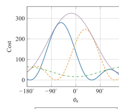
Figure 1 shows the values of f1 tof4dependent on the phase deviationφ=1φi−1φjin case that the virtual

mea-surements yi and yj have the same magnitudes as th

cor-respondent goals bi andbj. The values for bi=ej55

◦ and bj=2.3ej0

◦

have been chosen arbitrarily to yield cost func-tionals which plainly show the different behaviors. It can be seen that all four cost functionals have a minimum for φ=0◦. However, the cost functionalsf1andf2also show a false minimum for anotherφ6=0◦. For the case of no

mag-nitude deviations, i.e.ci=cj=1, the cost functionalf3is a scaled version of the cost functionalf4.

−180◦ ₋₉₀◦ ₀◦ ₉₀◦ ₁₈₀◦ 0

20 40 60

φ

Cost

f1 f2 f3 f4

Figure 1.Cost functionals for phase error only. For this example the goal values have been chosen to bebi=ej55

◦

andbj=2.3ej0

◦

.

−180◦ ₋₉₀◦ ₀◦ ₉₀◦ ₁₈₀◦

0 100 200 300

φ

Cost

f1 f2 f3 f4

Figure 2.Cost functionals with phase and magnitude error. For this example, additionally to the phase deviation, a multiplicative am-plitude deviation ofci=2.3 andcj=1.3 is assumed.

In the minimization process, while the minimization has not terminated yet, in general there will be phase deviations φ6=0 as well as magnitude deviations ci 6=cj6=1.

Fig-ure 2 shows the values of the cost functionals dependent on the phase deviationφ for virtual measurements which

de-viate from the goals in phase as well as in magnitude, viz. ci =2.3 and cj =1.3. The false minima forf1 andf2 are more distinct than in Fig. 1 and the cost functionalsf1 and f2can return zero and thus reach their global minimum even though neither magnitudes nor the phase difference matches the goals. The cost functionalsf3andf4have a minimum for a single value ofφonly, i.e. they do not suffer from false

(5)

For an analysis, the cost functionals f1tof4 can be ex-pressed in terms of their magnitude and phase deviation. For the cost functionalf1we have

f1=

β1−

yi+yj

2 2 = bi+bj

2 − cibie

j 1φi₊_c

jbjej 1φj

2 2 = |bi|

2₁₋_c2

i

+bj

2

1−c2_j

+2|bi|

bj

Re

n

ej φj i₋_c

1c2ej(φj i+1φi−1φj)

o 2 = |bi|

2₁₋_c2

i

+bj

2

1−c2_j

+2|bi|

bj

Re

n

ej φj i₋_c

1c2ej(φj i+8)

o

2

. (24) Accordingly, for the cost functionalf2we have

f2=

β2−

yi−j yj

2 2 = bi+j bj

2 − cibie

j 1φi₋_{j c}

jbjej 1φj

2 2 = |bi|

2₁₋_c2

i

+bj

2

1−c2_j

+2|bi|

bj

Im

n

ej φj i₋_c

1c2ej(φj i+φ)

o

2

. (25) The cost functionals f1 and f2 deviate from each other only by evaluating the real and imaginary part of ej φj i₋ cicjej(φj i+φ)respectively. Thus, they suffer from the same

kind of undesired behavior. For any given magnitude devia-tionciandcj, both cost functionals have two minima for two

different values ofφ(there are two numbers on the unit

cir-cle which have the same imaginary or real part respectively). The desired behavior would be that the cost functionals have a single minimum forφ=0 only. The occurring false

mini-mum reflects the fact that a single linear combination magni-tude does not uniquely define the phase difference between the two complex numbersbi andbj. Note, that two distinct

minima might occur for each of the cost functionalsf1and f2even, when the magnitudes|yi| = |bi|and

yj = bj are

equal to the desired magnitudes, i.e.c1=c2=1.

For the analysis of cost functional f3, we introduce the auxiliary variable

A= |bi|2

1−c2_i

+bj

2

1−c2_j

. (26)

By identifying Eq. (24) as the squared magnitude of the real part and Eq. (25) as the squared magnitude of the imaginary part of the same complex number,f3can be written as f3=f1+f2

=

(1+j ) A+2|bi| bj

ej φj i₋_c1c2ej(φj i+φ)

2

=

(1+j ) Ae

−j φj i₊₂_|_b

i| bj

1−c1c2ej φ

2

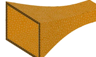
Figure 3.Mesh defining the RWG unknowns for transforming syn-thetic data of a horn antenna.

=

B−2|bi| bj

cicjej φ

2

(27)

with the auxiliary term B=(1+j ) Ae−j φj i₊₂_|_b

i|

bj

.

From the last row of Eq. (27) it is clear that the cost func-tionalf3 is minimal only for the single value of φ, when

it equals the phase ofBshifted by 180◦_{. The cost functional} obtains its minimum forci=cj=1 andφ=0, as intended,

however for general magnitude deviationsci 6=1 andcj6=1,

the cost functionalf3 may obtain its minimum atφ6=0.

Some tuples ci, cj, φ6=(1,1,0)can also lead tof3=0. However, together with the minimization of the magnitudes as described in Sect. 2, the cost functional has a unique global minimum (up to a global phase) foryi andyj.

The cost functionalf4can be rewritten in the form

f4=

β4−yiy

∗ j 2 = bib

∗

j−bib∗jcicjej φ

2

= |bi|2

bj 2

1−cicje

j φ

2

. (28)

The cost functionalf4has a global minimum forci=cj =1

andφ=0. Also independent on the deviation between yi

andbi andyj andbj, the minimum forf3occurs aφ=0.

However the cost functionalf3can return zero also for any combination of magnitude deviationsci=(1/cj)6=1. Thus

for a unique global minimum withci =cj =1 andφ=0

the cost functionalf3has to be minimized together with the magnitude cost functional from Sect. 2.

5 Numerical results

(6)

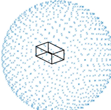
Figure 4.Location of the sample points.

is 227.40 mm×151.60 mm in size. The other side of the an-tenna builds a transition to a rectangular waveguide of dimen-sions 72.14 mm×34.04 mm. The horn length is 350 mm and the taper is a(1−cos)-taper. The excitations for the dipoles have been obtained approximately from a simulation in CST MICROWAVE STUDIO 2016 (CST, 2016). For the NFFFT the triangles on the same mesh has been used for RWG ba-sis functions (Rao et al., 1982), i.e. the vector zin Eq. (1) contains the coefficients of each RWG basis function.

As measurement probes serve Hertzian dipoles. Two probes at a time form a measurement pair which will be evaluated for the phase differences. A pair consists of two, horizontally separated dipoles spaced two wavelengths apart. The measurement points, i.e. the centers of the dipole pairs, are located on spirals on a spherical surface around the AUT. Figure 4 shows the 1000 locations of the pair centers along with a black cuboid denoting the location of the AUT. The spiral sampling shown in Fig. 4 is more uniformly distributed than the usual spherical sampling which has equidistant an-gular steps in ϑ andϕ direction. Since in general two in-dependent polarizations are needed in NF measurements, the same measurements have been obtained with rotated dipoles. Thus we have 4000 measurements (not counting any linear combinations) since at each measurement location two mea-surements – one to the left and one to the right – have been obtained with two polarizations. Any linear combination and phase differences can be obtained from the complex valued synthetic dipole outputs. In the following linear combina-tions and phase differences have been considered only for corresponding dipole pairs. Note, that the locations of dipoles of neighboring pairs do not interfere in general, which means that the absolute phases of the measurements at the individ-ual dipoles cannot be determined by iterating through a chain of known phase differences.

Table 1.Minimization overview.

Cost No. of ∅FF error max Time

iterations FF error

f 1285 −32.4 dB −14.9 dB 1.20 min

f+f1 1075 −36.4 dB −14.3 dB 1.14 min

f+f3 12 960 −81.9 dB −54.4 dB 10.92 min

f+f4 9493 −85.7 dB −62.2 dB 6.66 min

Four scenarios have been considered. In the first scenario, the coefficients inzare retrieved from magnitude only mea-surements as in Sect. 2. In the second scenario, additionally to the magnitudes of the single dipole outputs, the magni-tudes of the sum of the outputs of each dipole pair have been considered according to Sect. 3.1 and Eq. (24). In the third scenario also the magnitudes of the phase shifted sums have been considered as in Eq. (27). Finally, in the fourth scenario the phase knowledge has been included in terms of conju-gated multiplication as described in Sect. 3.2 and in Eq. (28). For all scenarios, the corresponding cost functional has been minimized with a L-BFGS procedure (Nocedal and Wright, 2006), a memory limited version of the Broyden–Fletcher– Goldfarb–Shanno algorithm (named after its inventors) in the family of quasi-Newton methods (Nocedal and Wright, 2006). The algorithm terminates, once an insufficient rela-tive decrease in the cost functional is observed. The initial conditions have been chosen to bezi=1+1j∀i for each

basis function in all scenarios. After the minimization has finished, the FF is calculated from the retrieved sources in z. Table 1 shows an overview over the four scenarios. The different timings are mostly due to the different number of iterations. All minimizations used roughly the same memory of about 450 MB. For Table 1, the complete FF has been con-sidered, not only the cuts which are shown in the following subsections.

5.1 Magnitude only measurements via cost functionalf

(7)

−180◦ ₋₉₀◦ ₀◦ ₉₀◦ ₁₈₀◦ −60

−40 −20 0

ϑ Eϑ

far

-fi

el

d

pa

tt

er

n

in

dB

Reference Retrieved Error

Figure 5.Retrieved FF from magnitude only data,ϕ=90◦.

0 500 1000

−40 −20 0

Iterations

Cost

functional

for

ﬁrst

scenario

in

dB

Figure 6.Progress of the minimization of the cost functional for magnitude only data.

shown in Table 1, the maximum FF error is at−14.9 dB and the average FF error is−32.4 dB.

5.2 Magnitudes of single measurements and of pair sums via cost functionalf+f1

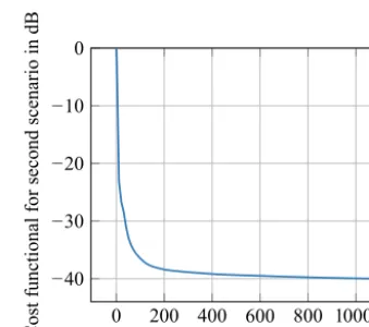
For the second scenario, also the magnitudes of the complex sum of the outputs of each dipole pair have been considered. The E-plane cut of the retrieved copolar FF component can be found in Fig. 7. The values in Table 1 suggest that there hardly is any improvement compared to the magnitude only minimization. Even though the retrieved FF in Fig. 7 seems to show a better result than Fig. 5, especially outside the main lobe, the error level is still very high and the minimization again seems to be captured at a local stationary point which is different from the one in the magnitude only minimization, even though the initial guess has been the same. This agrees with the analysis from Sect. 4, in which it was stated that false minima may occur for the additional cost functional parts in f1. Nevertheless, the usage of the magnitude of a

−180◦ ₋₉₀◦ ₀◦ ₉₀◦ ₁₈₀◦

−60 −40 −20 0

ϑ Eϑ

fa

r-fi

el

d

pa

tt

er

n

in

dB

Figure 7.Retrieved FF from magnitudes and one linear combina-tion data,ϕ=90◦.

0 200 400 600 800 1000

−40 −30 −20 −10 0

Iterations

Cost

functional

for

second

scenario

in

dB

Figure 8.Progress of the minimization of the cost functional for magnitude data combined with one linear combination magnitude per diploe pair.

linear combination has some effect since it leads to a termi-nation at a different stationary point than the magnitude only minimization. In some cases this may lead to a situation in which local stationary points from the magnitude only data are avoided. In this particular case, the minimization does not progress anymore after 1075 iterations, as shown in Fig. 8. 5.3 Magnitudes of single measurements, of pair sums, and of phase shifted pair sums via cost functional

f+f3

In the third scenario additionally to the magnitude only min-imization objectives also the two (squared) magnitudes of the linear combinationsbi+bj

2

andbi−j bj

2

have been considered for the dipole pairs. Figure 9 shows the retrieved copolar FF in the E-plane. With a maximum FF error of

(8)

−180◦ ₋₉₀◦ ₀◦ ₉₀◦ ₁₈₀◦

−60 −40 −20 0

ϑ Eϑ

fa

r-fi

el

d

patt

er

n

in

dB

Figure 9.Retrieved FF from magnitudes and two linear combina-tions data,ϕ=90◦.

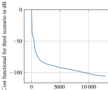
0 5000 10 000

−100 −50 0

Iterations

Cost

functional

for

third

scenario

in

dB

Figure 10.Progress of the minimization of the cost functional for magnitude data combined with two orthogonal linear combination magnitudes per dipole pair.

reached the minimum which corresponds to the correct near fields. This observations supports the conclusions of Sect. 4. The progression of the cost functional shown in Fig. 10 also shows that the minimization did not reach its minimal value before at least ten times the number of iterations of the first two scenarios but also shows a steady decrease. This suggests that all local stationary points have been avoided thanks to the additional objectives for the linear combinations. 5.4 Magnitudes of single measurements and

conjugated multiplication between pairs via cost functionalf+f4

In the fourth scenario, parallel to the magnitude only goals, the conjugated multiplications described in Sect. 3.2 have been minimized for the dipole pairs. Figure 11 shows the retrieved copolar FF pattern in the E-plane. Similar to the previous scenario, the retrieved FF coincides with the

ref-−180◦ ₋₉₀◦ ₀◦ ₉₀◦ ₁₈₀◦

−60 −40 −20 0

ϑ Eϑ

fa

r-fi

el

d

pa

tt

er

n

in

dB

Figure 11.Retrieved FF from magnitudes and conjugated multipli-cation data,ϕ=90◦.

0 2000 4000 6000 8000 10 000

−100 −50 0

Iterations

Cost

functional

for

fourth

scenario

in

dB

Figure 12. Progress of the minimization of the cost functional for magnitudes combined with conjugated multiplication data per dipole pair.

erence. As stated in Table 1, the maximum FF error is less than−60 dB. The retrieved FF as well as the progression in Fig. 12 suggest that any local stationary points have been avoided and the correct NF has been retrieved.

6 Conclusions

(9)

behave differently during the minimization procedure. When the phase goals are chosen with care, the cost functional ex-hibits a unique global minimum (up to a global phase) which corresponds to the fully restored radiated NF. From this re-stored NF, the FF can be computed easily with means of standard NFFFT. For the cost functionals with a global min-imum corresponding to the correct NF, the FF has been re-trieved with a maximum error of up to −62 dB. However, even though an unique global minimum exists for the radi-ated fields, the minimization may not converge to this mini-mum due to the non linearity of the problem. In such a case, the minimization runs into a local stationary point. Incorpo-rating phase knowledge can help to avoid stationary points in this case. This way, one can retrieve a barely distorted FF without the need of full phase measurements.

Data availability. Underlaying data is available from the corre-sponding author upon request.

Competing interests. The authors declare that they have no conflict of interest.

Disclaimer. The responsibility for the content of this publication is with the authors.

Acknowledgements. This work has been supported by the German Federal Ministry for Economic Affairs and Energy under Contract No. 50YB1512.

This work was supported by the German Research Foundation (DFG) and the Technische Universität München within the funding programme Open Access Publishing.

Edited by: R. Schuhmann

Reviewed by: two anonymous referees

References

Bauschke, H. H., Combettes, P. L., and Luke, D. R.: Phase retrieval, error reduction algorithm, and Fienup variants: a view from con-vex optimization, J. Opt. Soc. Am. A, 19, 1334–1345, 2002. Candes, E. J., Strohmer, T., and Voroninski, V.: Phaselift: Exact and

stable signal recovery from magnitude measurements via convex programming, Commun. Pur. Appl. Math., 66, 1241–1274, 2013. Candes, E. J., Li, X., and Soltanolkotabi, M.: Phase retrieval via Wirtinger flow: Theory and algorithms, IEEE T. Inform. Theory, 61, 1985–2007, 2015.

Costanzo, S. and Di Massa, G.: An integrated probe for phaseless plane-polar near-field measurements, Microw. Opt. Techn. Let., 30, 293–295, 2001.

Costanzo, S., Di Massa, G., and Migliore, M. D.: A novel hybrid approach for far-field characterization from near-field amplitude-only measurements on arbitrary scanning surfaces, IEEE T. An-tenn. Propag., 53, 1866–1874, 2005.

CST: CST MICROWAVE STUDIO 2016, available at: https://www. cst.com/products/cstmws (last access: 28 March 2017), 2016. Eibert, T. F. and Schmidt, C. H.: Multilevel fast multipole

acceler-ated inverse equivalent current method employing Rao–Wilton– Glisson discretization of electric and magnetic surface currents, IEEE T. Antenn. Propag., 57, 1178–1185, 2009.

Eibert, T. F., Kilic, E., Lopez, C., Mauermayer, R. A., Neitz, O., and Schnattinger, G.: Electromagnetic Field Transformations for Measurements and Simulations (Invited Paper), Prog. Electro-magn. Res., 151, 127–150, 2015.

Fienup, J. R.: Phase retrieval algorithms: A comparison, Appl. Op-tics, 21, 2758–2769, 1982.

Gerchberg, R. W.: A practical algorithm for the determination of phase from image and diffraction plane pictures, Optik, 35, 237– 246, 1972.

Netrapalli, P., Jain, P., and Sanghavi, S.: Phase retrieval using alter-nating minimization, Adv. Neur. In., 2796–2804, 2013. Nocedal, J. and Wright, S.: Numerical optimization, 2nd Edn.,

Springer Science & Business Media, 2006.

Rao, S., Wilton, D., and Glisson, A.: Electromagnetic scattering by surfaces of arbitrary shape, IEEE T. Antenn. Propag., 30, 409– 418, 1982.

Schmidt, C., Schobert, D., and Eibert, T.: Electric dipole based synthetic data generation for probe-corrected near-field antenna measurements, in: Proceedings of the 5th European Conference on Antennas and Propagation (EUCAP), 3269–3273, 2011. Schmidt, C. H., Leibfritz, M. M., and Eibert, T. F.: Fully

probe-corrected near-field far-field transformation employing plane wave expansion and diagonal translation operators, IEEE T. An-tenn. Propag., 56, 737–746, 2008.

Schnattinger, G., Lopez, C., Kiliç, E., and Eibert, T. F.: Fast near-field far-field transformation for phaseless and irregular antenna measurement data, Adv. Radio Sci., 12, 171–177, https://doi.org/10.5194/ars-12-171-2014, 2014.

Waldspurger, I., d’Aspremont, A., and Mallat, S.: Phase recov-ery, maxcut and complex semidefinite programming, Math. Pro-gram., 149, 47–81, 2015.

Wu, X., Liu, H., and Yan, A.: X-ray phase-attenuation duality and phase retrieval, Opt. Lett., 30, 379–381, 2005.

Yurtsever, A., Hsieh, Y.-P., and Cevher, V.: Scalable con-vex methods for phase retrieval, in: 2015 IEEE 6th In-ternational Workshop on Computational Advances in Multi-Sensor Adaptive Processing (CAMSAP), IEEE, 381–384, https://doi.org/10.1109/CAMSAP.2015.7383816, 2015. Zhang, H. and Liang, Y.: Reshaped Wirtinger Flow and