Multirate PWM balance method for the efficient field-circuit coupled simulation of power converters

(1)

R E S E A R C H

Open Access

Multirate PWM balance method for the

efﬁcient ﬁeld-circuit coupled simulation of

power converters

Andreas Pels

1,2,3*

_{, Herbert De Gersem}

1,2

_{, Ruth V. Sabariego}

3

_{and Sebastian Schöps}

1,2

*_{Correspondence:} [email protected] 1_{Graduate School of Computational}

Engineering, Technische Universität Darmstadt, Darmstadt, Germany

2_{Institut für}

Teilchenbeschleunigung und Elektromagnetische Felder, Technische Universität Darmstadt, Darmstadt, Germany

Full list of author information is available at the end of the article

Abstract

The field-circuit coupled simulation of switch-mode power converters with conventional time discretization is computationally expensive since very small time steps are needed to appropriately account for steep transients occurring inside the converter, not only for the degrees of freedom (DOFs) in the circuit, but also for the large number of DOFs in the field model part. An efficient simulation technique for converters with idealized switches is obtained using multirate partial differential equations, which allow for a natural separation into components of different time scales. This paper introduces a set of new PWM eigenfunctions which decouple the systems of equations and thus yield an efficient simulation of the field-circuit coupled problem. The resulting method is called the multirate PWM balance method.

Keywords: Finite element methods; Numerical analysis; Partial diﬀerential equations; Linear circuits; DC-DC power conversion

1 Introduction

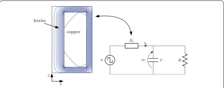
Switch-mode power converters are used in various devices from small-scale applications like mobile phone chargers to industrial large-scale applications like welding devices [7]. These converters use transistors to switch on and off the input voltage to produce an output voltage, which, in average, has the desired amplitude. A filter circuit is used to smoothen the output. The simulation of these devices is computationally expensive since, through the transistor switching, steep transients occur in the converter. Furthermore of-ten a switch-event detection is necessary to avoid step size rejection or even solver failures [14]. A multirate method has been developed in [9,10] which uses the concept of Multi-rate Partial Differential Equations (MPDEs) [3,12] and a combination of a Galerkin ansatz and conventional time discretization to efficiently solve problems with pulsed excitation. The method is applicable to power converters in which the switching behavior is idealized and known a-priori. It is particularly efficient in the case of linear elements. Some circuit elements may only be accurately represented by field models. For example the induced currents in the conducting materials of an inductor usually cause eddy current losses, which can easily be accounted for in a field model but not in a circuit model. In this paper the multirate method from [9,10] is applied to a linear buck converter circuit (see Fig.1) in which the inductor is represented by a 2D finite element model. This substantially

(2)

Figure 1Simpliﬁed circuit of the buck converter in continuous conduction mode withC= 10μF and

R= 30Ω. The ﬁeld model of the pot inductor (axisymmetric aroundz-axis) is designed to have an inductance ofL= 65 mH and a series resistance ofRL= 800 mΩat DC. The ﬁgure shows the equipotential lines of the

magnetic vector potential

creases the size of the strongly coupled system of equations. To still ensure an efficient simulation, a basis transformation is applied to the pulse-width modulation (PWM) basis functions [5] leading to decoupled systems of equations which can be solved efficiently in parallel. The resulting method is called the multirate PWM balance method in analogy with the harmonic balance method where harmonic functions take the place of the PWM basis functions. Numerical results on the buck converter show the efficiency and accuracy of the proposed method in field-circuit coupled problems.

The paper is structured as follows. Section2introduces the concept of MPDEs and ex-plains the solving procedure using Galerkin approach and conventional time discretiza-tion. Subsequently Sect.3presents the original PWM basis functions as described in [5]. In Sect.4the PWM eigenfunctions are developed and their advantageous properties for the solving process are highlighted. Finally Sect.5summarizes numerical results and com-pares the three diﬀerent solution approaches, i.e., conventional time discretization and the MPDE approach with PWM basis functions on the one hand and PWM eigenfunctions on the other hand. The paper is concluded by summarizing its content in Sect.6.

2 Multirate formulation

Let the field-circuit coupled model [13] of the converter be described by the system of ordinary differential or differential-algebraic equations

A d

dtx(t) + B x(t) = c(t), (1)

where A∈RNs×Ns _{is a possibly singular matrix, B}∈RNs×Ns _{is assumed to be a regular} matrix, x(t)∈RNs _{is the unknown solution, c(t)}∈RNs _{is the excitation, and}_t∈_(0,T_{] is} the simulation interval. The initial state of the model is given by consistent [6] initial values

x(0) = x0. The ideal pulsed excitation

vi(t) = ⎧ ⎨ ⎩

V0 for allτ(t)≤D,

(3)

is used as input of the power converter circuit. We denote byτ(t) =_Tt

s modulo 1 the rela-tive time,Tsis the switching cycle andDis the duty cycle.

The system of Multirate Partial Diﬀerential(-Algebraic) Equations (MPDEs or MPDAEs) with two time scales corresponding to (1) is given by [3,11,12]

A

∂x

∂t1

+ ∂x ∂t2

+ Bx(t1,t2) =c(t1,t2), (3)

wherex(t1,t2) is the unknown multivariate solution andc(t1,t2) is the multivariate

ex-citation. Choosing the multivariate excitation such thatc(t,t) = c(t), the solution of (1) and (3) are related byx(t,t) = x(t). Thus, the solution of (1) can be calculated solving the MPDEs and extracting the solution along a diagonal through the computation domain. To solve the MPDEs, additional conditions need to be speciﬁed. For the present applica-tion, a combination of initial and boundary values is applied. Initial values are supplied by

x(0,t2) = h(t2), i.e., att1= 0, where h with h(0) = x0is a function deﬁning the initial values

for allt2. The solution along the fast time scalet2is periodic, i.e.,x(t1,t2+Ts) =x(t1,t2).

The multivariate right-hand side is chosen asc(t1,t2) = c(t2), i.e., the pulses of the

excita-tion occur along the fast time scale. It is possible to use MPDEs with more than two time scales. However, in the applications of this paper, it is not necessary and furthermore often not feasible since the dimension of the computation domain increases and thus also the computational eﬀort to calculate the solution.

To solve the MPDEs (3), a Galerkin approach and time discretization is applied [2,10]. Thej-th solution componentxj(t1,t2) is approximated by expanding it into periodic basis

functionspkdepending on the fast time scalet2 and coeﬃcientswj,k depending on the

slow time scalet1

x_jh(t1,t2) := Np

k=0

wj,k(t1)pk τ(t2)

, (4)

where the periodicity of the basis functions is accounted for by using the relative time τ(t2) =_Tt2_s modulo 1. Applying the Galerkin approach with respect tot2and over one

pe-riod of the excitation [0,Ts] leads to

Adw dt1

+Bw(t1) =C(t1), (5)

with block matricesA=J ⊗A,B=J ⊗B+Q⊗A, where

J =Ts

1

0

¯

p(τ) p(τ) dτ, Q= –

1

0

dp¯(τ) dτ p

₍_τ_{) d}_τ_, ₍₆₎

and right-hand side

C(t1) =

Ts

0

¯

p τ(t2)

⊗c(t1,t2) dt2. (7)

¯

(4)

Figure 2Original PWM basis functionspk(τ),k∈ {0, 1, 2, 3, 4}

3 PWM basis functions

The PWM basis functions developed in [5] are built up starting from the zero-th constant basis functionp0(τ) = 1 and the piecewise linear basis function

p1(τ) = ⎧ ⎨ ⎩

√ 32τ–D

D if 0≤τ<D,

√

31+_1–D–2_Dτ ifD≤τ≤1, (8)

which includes the duty cycleDof the excitation by construction. The higher-order basis functionspk(τ), 2≤k≤Npare recursively obtained by integrating the basis functions of

lower orderpk–1(τ) and orthonormalizing them using the Gram–Schmidt algorithm. The

generated basis functions are depicted in Fig.2.

For the PWM basis functions, the matricesJ andQfrom (6) are given byTsmultiplied

by the identity matrix (due to the orthonormality of the basis functions) and a square matrix with around 25% of non-zero entries, respectively. Solving the problem requires time stepping of the entire system (5).

4 PWM eigenfunctions

To enable an easy parallelization of the method, the equations (5) can be decoupled, for example by diagonalizingQ, i.e., a basis transformation. We deﬁne new basis functions gk(τ) as linear combinations of the PWM basis functions, i.e.,

gk(τ) := Np

l=0

vk,lpl(τ), (9)

wherevk,lare unknown coeﬃcients withk∈ {0, . . . ,Np}, andgk(τ) are eigenfunctions of

the time derivative operator

d

dτgk(τ) =λkgk(τ). (10)

We enforce this property in a weak sense by a Galerkin approach, i.e.,

–

1

0

gk(τ)

dpm(τ)

dτ dτ=λk

1

0

(5)

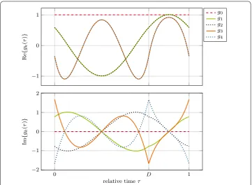
Figure 3PWM eigenfunctionsgk(τ),k∈ {0, 1, 2, 3, 4}, i.e.,Np= 4. (top) real part. (bottom) imaginary part

where integration by parts and the periodicity of the basis functions is used. Inserting the expansion of the basis functions into (11) gives

TsQvk=λkJvk. (12)

SinceJ isTsmultiplied by the identity matrix (thanks to the orthonormality of the PWM

basis functions), the λk and vk are the eigenvalues and eigenvectors of the matrix Q,

respectively. Furthermore since Qis real-valued and skew symmetric, and therefore a normal matrix, the eigenvectors vkare orthonormal. The new basis functions

(complex-valued) are depicted in Fig.3forNp= 4. Note that the basis consists of pairs of conjugate

complex basis functions.

Inserting the transformed basis functions instead of the PWM basis functions into (6) and (7) leads, using the orthonormality of the eigenvectors, to

Adw dt1

+Bw(t1) =C(t1), (13)

whereAas in (5),

B=J ⊗B+Λ⊗A, (14)

C(t1) =

Ts

0

¯

g τ(t2)

⊗c(t1,t2) dt2, (15)

(6)

leads toNp+ 1 independent systems of equations given by

TsA

dwk

dt1

+ (TsB+λkA) wk=

Ts

0

¯ gk τ(t2)

c(t1,t2) dt2 fork= 0, . . . ,Np, (16)

where w = [w₀, w₁, . . . , w_N_p]. Note that if a diagonal entry inΛis complex, there is also a complex conjugate counterpart. The solutions of the decoupled system of equations cor-responding to this complex eigenvalue and its conjugate complex counterpart, are, as a result, complex conjugate to each other. Therefore it is suﬃcient to solve one of them. This is similar to harmonic balance methods in which the harmonic basis functions are given by pairs of complex conjugates leading to similar systems of equations. In analogy to “harmonic balance method”, we call the developed method the “multirate PWM balance method”.

5 Test case and numerical results

The method is applied to the buck converter from Fig.1, where the pot inductor is repre-sented by a 2D ﬁeld model with conducting core material (ferrite,σfe= 250 S/m). The coils

are modeled as stranded conductors. The simulation interval is given byΨ = [0, 10] ms. The switching frequency isfs=_T1_s = 1000 Hz. For the pulsed excitation (2) we useV0=

24 V. All calculations are performed in MATLAB. The partial diﬀerential equations gov-erning the magnetoquasistatic problem are given by

σ(r)∂Am(r,t) ∂t +∇ ×

μ(r)–1∇ ×Am(r,t)

= Js(r,t), (17)

where r is the position vector,tis the time, Amis the modiﬁed magnetic vector

poten-tial [4], Jsare the imposed currents,μ= 4π×10–7H/m is the magnetic permeability and

σ is the conductivity which is only non-zero in the ferrite core (σfe). The problem is

con-sidered on a 2D planar domain with homogeneous Dirichlet boundary conditions. Correspondingly, the Finite Element magnetoquasistatic [13] discretization of the mag-netoquasistatic inductor model is given by the diﬀerential-algebraic system of equa-tions [8]

Mσ d

dta(t) + K a(t) = PiL(t), (18)

where Mσ is the singular conductivity matrix, K is the stiﬀness matrix, a(t) gathers the degrees of freedom (DOFs) related to the magnetic vector potential, P is the discretiza-tion of the winding funcdiscretiza-tion [13] andiL(t) is the current through the inductor. The

field-circuit coupling is expressed as follows. An additional variable is introduced for the mag-netic flux linkageΦ(t) = Pa(t). All equations are coupled monolithically into the index-1 differential-algebraic system of equations [1]

Mσ d

dta– PiL+ K a = 0, (19)

Pa–Φ= 0, (20)

d

(7)

C d

dtvC–iL+ 1

RvC= 0, (22)

which for the example in Fig.1contains a total of 11,053 DOFs. The initial conditions are given byvC(0) = 0,iL(0) = 0 and a(0) = 0.

The initial condition for the MPDEs (3) can be written as

hj(t2)≈ Np

k=0

wj,k(0)pk τ(t2)

, (23)

wherehjis thej-th element of h. It only has to satisfy the condition h(0) =x(0, 0) = x0.

Consequently there is a high degree of freedom in choosing the initial values w(0) for the system of equations (5). However not all choices lead to an eﬃcient simulation, i.e., low dynamics in the slow time scale. The following choice of initial values has proven advantageous. First, the steady-state solution is calculated, i.e.,

ws=B–1C(0). (24)

Secondly, the initial coeﬃcients fork= 1, . . . ,Npare extracted from the steady-state

solu-tionwj,k(0) =wjs,kfor allj. The remaining coeﬃcients are calculated by solving the solution

expansion (4) forwj,0(0) and using the conditionx(0, 0) = x0. In summary the initial

coef-ﬁcients are given by

wj,k(0) =

⎧ ⎨ ⎩

ws

j,k fork= 1, . . . ,Npand for allj= 1, . . . ,Ns,

xj(0) –

Np

l=1wjs,lpl(0) fork= 0 and for allj= 1, . . . ,Ns.

(25)

The initial conditions for the system of equations (13) are computed similarly using the PWM eigenfunctions. Other choices of initial values may still lead to the correct solution but might impair the eﬃciency of the method.

To calculate the reference solution with a conventional adaptive time discretization, the MATLAB solverode15sis used. It is modified to restart the simulation at the known switching instances. Consistent initial values for the restart of the solver are calculated by using a Newton–Raphson algorithm to solve the set of algebraic equations. The required differential variables are taken from the solution at the end of the prior solution interval. After finding the new set of initial values, the initial slopes of the differential variables are calculated by solving the subsystem of ordinary differential equations for the slope.

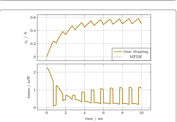
The multivariate solutionx(t1,t2) calculated using the multirate PWM balance method,

i.e., solving (13) withode15s, is reconstruced using (4) and the multivariate voltage at the capacitor is depicted in Fig.4. The corresponding solution component of the original system of equations (1) is extracted along a diagonal through the computation domain. Figure5shows the current through the inductor along with the reference solution. The agreement between the multirate PWM balance method solution and the reference solu-tion is excellent. The Joule losses in the core material due to eddy currents are calculated by

Peddy(t) =

Ω

(8)

Figure 4Multivariate voltage at the capacitor calculated using the multirate PWM balance method. The solution component corresponding to the original system of equations (1) is extracted along a diagonal and marked as a black curve

Figure 5(top) Reference solution calculated using conventional adaptive time discretization compared to the solution obtained by the MPDE approach withNp,pwmbal= 4 PWM eigenfunctions. The relativeL2error of

the current through the inductor similar to (27) is approximately 3×10–5_{. (bottom) Joule losses in the core}

material due to eddy currents

where E is the electric ﬁeld strength,Ωis the spatial computation domain, the superscript H denotes the Hermitian, i.e., the complex conjugate transposed, and e(t) = –d

dta(t) is the

line-integrated discrete electric ﬁeld. The Joule losses are plotted as well in Fig.5. Figure6 depicts the solution of (13), i.e., the coeﬃcients w(t1), exemplary for the current through

the inductoriL. As one can see, using the initial values (25), only the coeﬃcientwj,0

(9)

conven-Figure 6Coeﬃcientsw1,kfor the inductor current calculated by solving (13) withNp,pwmbal= 4. (top) real

part. The coeﬃcientsw1,1,. . .,w1,4are approximately the same therefore they are hard to distinguish visually.

(bottom) imaginary part

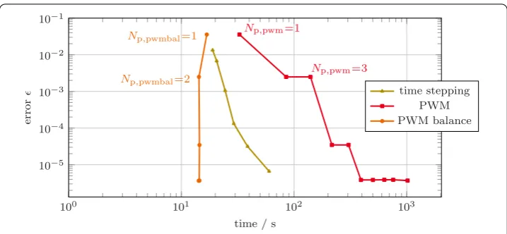
tional time discretization and to the MPDE approach with the original PWM basis func-tions. Diﬀerent settings are considered: To analyze the performance of the conventional time discretization, the relative and absolute tolerance setting of the solver is changed, i.e., abstol = reltol∈[10–6, 10–1]; For the case of the multirate PWM balance method and the MPDE approach with the original PWM basis functions, relative and absolute toler-ances are ﬁxed at abstol = reltol = 10–7and the number of basis functionsNp∈ {1, . . . , 10}

is changed. The accuracy is measured for the voltage output of the converter, i.e., the volt-age at the capacitor. The relative L2error is given by

(tol,Np) =

vC,ref(t) –vCh(tol,Np,t) L2₍_Ψ₎ vC,ref(t) L2₍_Ψ₎

, (27)

wherevC,refis the reference solution andvChis the solution using the multirate PWM

bal-ance method and the MPDE approach with the original PWM basis functions. The norm is approximated using mid-point quadrature. Figure7shows the error plotted as a function of the solution time, i.e., the time thatode15sneeds. For conventional time discretiza-tion the time for solving consists of the time that is needed to calculate consistent initial values and slopes after switching, and the actual time thatode15sneeds. The time to calculate consistent initial values and slopes depends on the number of switching instants and is thus constant if the switching frequency or simulation interval does not change. It is given by approximately 16 seconds. The total time displayed in Fig.7is the sum of both contributions.

(10)

Figure 7Erroras deﬁned in (27) over time for solving the systems of equations. The MPDE approach with PWM eigenfunctions (multirate PWM balance method) is considerably faster than the MPDE approach with the original PWM basis functions and the conventional time discretization

large systems of equations (1) (due to ﬁeld-circuit coupling) are even further increased in size through the Galerkin approach. The stagnation of the error at 10–6 _{in Fig.}₇_for

values larger thanNp= 7 is caused by the chosen accuracy ofode15s. Furthermore one

can see that when adding another basis function the error does decrease with every sec-ond basis function. This was already observed in [5,10]. For this reason the error for the PWM eigenfunctions is only plotted forNp,pwmbal∈ {1, 2, 4, 6, 8, 10}. Since the systems of

equations resulting from the multirate PWM balance method are decoupled, they can be solved eﬃciently in parallel. For each basis functiongkwithk= 0, . . . ,Np, a

complex-valued initial value problem of the form (16) has to be solved. The size of these systems of equations is the same as that of the original system of equations (1). However, the time for solving is considerably smaller since less time steps are necessary for the same solution accuracy. Note that due to the choice of the initial values (25) most coeﬃcients in (13) for this numerical example do not change and only those corresponding to the zero-th basis function vary. This means that only the decoupled system of equations which corresponds to the zero-th basis function takes considerable computational eﬀort to solve. In a paral-lel computing environment one would choose as many processor cores as basis functions (Np+ 1). The overall runtime is then determined only by the initial value problem that

takes the longest to integrate. For this numerical example it isk= 0. The communication overhead between processors is not taken into account since it is highly implementation and machine dependent. The slightly decreasing time to solution whenNp,pwmbal> 1 is

owed to the fact that initial values according to (25) take more a-priori information into account which leads to smaller number of time steps and faster simulation. The overall accuracy of the method is problem-speciﬁc and always depends on both the tolerance for the solver and the number of basis functions. An a-priori determination of the number of basis functions and the solver tolerance is not yet available. An a-posteriori estimator can be constructed by increasing the number of basis functions and comparing the solutions. The resulting error is also related to the time stepping error.

(11)

repre-sent the solution of problems with nonlinear elements [10]. If the amplitude of the ripples is small compared to the amplitude of the envelope, the particular eﬃcient approach de-scribed in [9] can be applied. It uses only the slowly varying envelope to evaluate the non-linearities. Although the assembly of the ﬁeld model matrices for a new envelope cannot be parallelized, the matrices in (13) can still be decoupled and calculations to obtain the following time step can be run in parallel.

6 Conclusion

A new efficient technique was presented for field-circuit coupled models of DC-DC power converters, in which the switches are idealized and the filtering circuit is linear. The already existing MPDE technique with PWM basis functions splits the solution into fast varying and slowly varying parts. In this paper this method has been improved by introducing a new set of PMW basis functions which decouple the systems of equations similar as in the harmonic balance method. The new method, now called multirate PWM balance method, enables a parallel solution of all PWM modes resulting in a speed-up amounting to a factor 4 for the test example.

Acknowledgements

This work is supported by the “Excellence Initiative” of German Federal and State Governments and the Graduate School CE at TU Darmstadt. The authors thank Johan Gyselinck for fruitful discussions. Further thanks go to Jonas Bundschuh and Erik Skär for their contribution to the ﬁrst implementation of the PWM eigenfunctions.

Funding

No funding to report.

Abbreviations

DOFs, degrees of freedom; PWM, pulse-width modulation; MPDE, multirate partial diﬀerential equation.

Availability of data and materials

Not yet available publicly. It is, however, planned to make the code, which is used to generate the results, publicly available in the near future.

Competing interests

There are no competing interests to report.

Authors’ contributions

All authors have jointly carried out the research and worked together on the manuscript. The numerical tests have been conducted by the ﬁrst author. All authors read and approved the ﬁnal manuscript.

Author details

1_{Graduate School of Computational Engineering, Technische Universität Darmstadt, Darmstadt, Germany.}2_{Institut für}

Teilchenbeschleunigung und Elektromagnetische Felder, Technische Universität Darmstadt, Darmstadt, Germany.

3_{Department of Electrical Engineering, EnergyVille, KU Leuven, Leuven, Belgium.}

Publisher’s Note

Springer Nature remains neutral with regard to jurisdictional claims in published maps and institutional aﬃliations.

Received: 20 May 2019 Accepted: 11 July 2019

References

1. Bartel A, Baumanns S, Schöps S. Structural analysis of electrical circuits including magnetoquasistatic devices. Appl Numer Math. 2011;61:1257–70.https://doi.org/10.1016/j.apnum.2011.08.004.

2. Bittner K, Brachtendorf HG. Adaptive multi-rate wavelet method for circuit simulation. Radioengineering. 2014;23(1):300–7.

3. Brachtendorf HG, Welsch G, Laur R, Bunse-Gerstner A. Numerical steady state analysis of electronic circuits driven by multi-tone signals. Electr Eng. 1996;79(2):103–12.https://doi.org/10.1007/BF01232919.

4. Emson CRI, Trowbridge CW. Transient 3d eddy currents using modiﬁed magnetic vector potentials and magnetic scalar potentials. IEEE Trans Magn. 1988;24(1):86–9.https://doi.org/10.1109/20.43862.

5. Gyselinck J, Martis C, Sabariego RV. Using dedicated time-domain basis functions for the simulation of pulse-width-modulation controlled devices – application to the steady-state regime of a buck converter. In: Electromotion 2013. Romania: Cluj-Napoca; 2013.

(12)

6. Lamour R, März R, Tischendorf C. Diﬀerential-algebraic equations: a projector based analysis. Diﬀerential-algebraic equations forum. Heidelberg: Springer; 2013.https://doi.org/10.1007/978-3-642-27555-5.

7. Mohan N, Undeland TM, Robbins WP. Power electronics: converters, applications and design. 3rd ed. New York: Wiley; 2003.

8. Nicolet A, Delincé F. Implicit Runge–Kutta methods for transient magnetic ﬁeld computation. IEEE Trans Magn. 1996;32(3):1405–8.https://doi.org/10.1109/20.497510.

9. Pels A, Gyselinck J, Sabariego RV, Schöps S. Solving nonlinear circuits with pulsed excitation by multirate partial diﬀerential equations. IEEE Trans Magn. 2018;54(3):1–4.https://doi.org/10.1109/TMAG.2017.2759701.

10. Pels A, Gyselinck J, Sabariego RV, Schöps S. Eﬃcient simulation of DC-DC switch-mode power converters by multirate partial diﬀerential equations. IEEE J Multiscale Multiphys Comput Tech. 2019;4(1):64–75.

https://doi.org/10.1109/JMMCT.2018.2888900.

11. Pulch R, Günther M, Knorr S. Multirate partial diﬀerential algebraic equations for simulating radio frequency signals. Eur J Appl Math. 2007;18(6):709–43.https://doi.org/10.1017/s0956792507007188.

12. Roychowdhury J. Analyzing circuits with widely separated time scales using numerical PDE methods. IEEE Trans Circuits Syst I, Fundam Theory Appl. 2001;48(5):578–94.https://doi.org/10.1109/81.922460.

13. Schöps S, De Gersem H, Weiland T. Winding functions in transient magnetoquasistatic ﬁeld-circuit coupled simulations. Compel. 2013;32(6):2063–83.https://doi.org/10.1108/COMPEL-01-2013-0004.