*Correspondence:
doktor@mathematik.uni-kl.de
1Mathematics Department,
Technische Universität Kaiserslautern, Kaiserslautern, Germany
2Department of Civil Engineering,
Technische Universität Kaiserslautern, Kaiserslautern, Germany
Abstract
Non-destructive testing methods became popular within the last few years. For steel beams incorporated in buildings there are currently only destructive ways for testing the yield limit as well as for determination of the current stress level. Rise of ultrasonic and micro-magnetic tools for (non-destructive) measurements allows the
characterization of the inbuilt material especially of old steel bridges as economical maintenance of the infrastructure. It is possible to determine the reserve of residuence of bridges or of any other existing steel buildings in order to upgrade them competitively for future usage by the possibility of a simple way of strengthening by welding or using bolds. This is done using modern devices for ultrasonic and micro magnetic data recording on the one hand and modern techniques from nonparametric statistics such as sieve, partition and semi-recursive estimators on the other hand.
Keywords: Nonparametric regression; Robust regression; Mathematical and mechanical modeling; Dependency modeling; Civil engineering; Non-destructive testing; Material characterization
1 Introduction
The load bearing capacity in existing buildings is classically determined by means of load tests. If a calculation model gives no sufficient results, highly complex test loadings have to be done to determine the load bearing capacity. For verification in existing buildings material characteristics as the yield strength and the existing stresses have to be known, determining them non-destructively is an obvious advantage. Furthermore, the internal forces could be estimated, which includes second order theory as well as e.g. imperfections and signal denoising (outlier detection). This is crucial for the verification of (sufficient) load bearing capacity. The appointed lifetime of a new building is 50 to 100 years. Es-pecially for steel buildings, with high variations but well known material characteristics, extensions of the lifetime in the sense of sustainability might be possible, cf. [1]. The actual standards for condition monitoring are in [2,3] with [4,5] explaining how to localise fa-tigue effects before crack initiation starts. Therewith mechanical stresses can be obtained via electromagnetic induced ultrasonic measurements and acusto-elastic effects, cf. [6,7]. Thus, mathematical modeling is necessary for the micromagnetic records to determine material characteristics, the ultrasonic records to determine the current state of load and finally generalising the mechanical model to estimate the internal forces. This work links
the non-destructive records with modeling and the generally accepted engineering stan-dards.
2 Non-destructive testing methods
To determine the residual carrying capacity of a construction without risk of collapse is just possible with non-destructive testing methods. The determination of the yield strength by micromagnetic measurements and the determination of the current load state by ultrasonic measurements are described below.
2.1 Unknown material characteristics
The yield strength is the most important material characteristic of the steel to determine the load-bearing capacity. It is defined via regulations to characterize different steel qual-ities. If the yield limit is determined by measurements, the ultimate limit state design can be proven by real material characteristics without model uncertainties and not by guaran-teed minimum values. For determination of the yield strength of an investigated beam the ferromagnetic properties of steel are used. There is a causal relation between magnetism and the yield limit to be determined, see [8] for details. For calibration means, the mag-netic properties of the different steel types are determined and assigned to their yield limit measured in a classical tensile test.
2.2 Determination of the current load state
The determination of the current state of stress of a built-in steel beam is possible via ultra-sonic measurements, compare [7,9,10]. The influence of the stress and strain conditions on the speed of the propagation of the ultrasonic waves is used for the ultrasonic stress analysis. Comparing the speed of the ultrasonic waves in a beam without loadv0and the speed in a beam with loadvl, the current state of stressς(inmmN2) can be determined using
the following equation:
ς=(v0–vl)
v0 ·K
H, (1)
K
H is a linear factor, a so-called acusto-elastic constant, that is determined in lab tests,
compare Fig.1. In these tests the speedv0is measured in beams without load. In practice, there is no possibility for a direct measurement as there are no in-built beams without load. Due to the anti-symmetric stress distribution in the cross section of a beam, the speedv0can be determined by the mean value of symmetrically distributed measurement
Figure 2Left:Speed variation influenced by stress.Right:Speed variation due to texture
points in a loaded beam assuming that there is no axial force. The texture due to the rolling process of a steel beam causes the directional property of the ultrasonic measuring results (anisotropism). The difference of the speed according to the texture is shown in Fig.2,
Right and the difference of the speed according to the stress due to loading is shown in Fig.2,Left. Ultrasonic measurement values are the addition of both of them. The influence of texture is up to ten times higher than the influence of stresses. To show a sufficient bearing resistance, the much greater influence of texture has to be eliminated.
3 Construction & measurements in existing buildings
3.1 Construction
Higher static loads can easily be supported by steel constructions with simple strength-ening measures. But the used steel and its material characteristics, especially his bearing capacity, are not known. Furthermore, the current state of load is typically unknown. Mod-ifications of buildings in their previous service lifes caused changed load transfers, which are not incorporated in current construction plans. In many cases, construction plans of the building to be investigated do not exist anymore. Thus, it is impossible to make a se-rious statement about the load bearing capacity still available in the beams.
3.2 Recording data
Recording data in an existing building is a grueling task which has to be improved. The measurement equipment needs external electrical power supply and should be adapted to run with a battery to make it more handy, unless the devices themselves are quite small and handy, compare Fig.3and Fig.4. Nevertheless, measurements have been made at the materials testing institute (MPA) of the University of Kaiserslautern as well as in exist-ing buildexist-ings like the Ceasarparkbrücke (Kaiserslautern), see Fig.5, and a covered market (Frankfurt/Main), see Fig.4. In the sequel, the data evaluated in Sect.5are those obtained in the lab test because the exact load situation is known, thus, we have structural as well as measured residuals for the evaluation of the techniques.
4 Mathematical modeling and applications
Figure 3Left:Both sensors for recording ultrasonic runtimes and micromagnetic.Right:A coated steel beam in the lab with devices to record ultrasonic signals as well as micromagnetic quantities. The notebook in front shows hysteresis curves surveilling the micromagnetic records used for the determination of the yield strength
Figure 4Left:An AScan which gives, via peak-to-peak-analysis, the time-of-flight of the ultrasonic waves to estimate the stress.Right:Recording data in the market hall
Figure 5Left:The Caesarparkbrücke in Kaiserslautern.Right:Optimal Measurement Conditions on coated beam
Figure 6Left:The 7 traces times-of-flight are recorded in as a cross section (compare Abb. 5.25 in [9]).Right:
An overview about the amount of beams and, thus, complexity of records and changes of the statical system
4.1 Mathematical and mechanical models
The stresses existing in a steal beam can be decomposed in different sources of stress via classical/technical mechanics, see e.g. [9]. For security and safety concepts, we have to decompose them in their single parts: normal (N) and residual (E) stress, stress due to bending around theyorzaxis (MyandMz, respectively) and stress due to warping torsion
(Mw). The concept of measuring points uses symmetry as far as possible and looks, locally
in every cross section of the steel beam along the x-axis, as follows:
This leads to the following identities for the local stresses which has to be handled math-ematically, compare Fig.6and [14] for details:
ς1(x) =
z1
iy
My(x) +
y1
iz
Mz(x) +
q1
iw
Mw(εx) +E1+N, (2)
ς2(x) =
z2
iy
My(x) +
y2
iz
Mz(x) +
q2
iw
Mw(εx) +E2+N, (3)
ς3(x) =
z3
iy
My(x) +E3+N, (4)
ς4(x) =E4+N, (5)
ς5(x) =
z5
iy
My(x) +E5+N, (6)
ς6(x) =
z6
iy
My(x) +
y6
iz
Mz(x) +
q6
iw
Mw(εx) +E6+N, (7)
ς7(x) =
z7
iy
My(x) +
y7
iz
Mz(x) +
q7
iw
Mw(εx) +E7+N (8)
with known constants from geometry:ε,iy,iz,iw,zj,yj,qj,j= 1, . . . , 7. We will usegi=
(gyi,gzi,gwi) = (
zi
iy,
yi
iz,
qi
iw) in Sect.4.3to shorten notation. Assume the bending moments
My,Mz to be polynomials of degree at mostn∈Nand the warping torsion to be some
hyperbolic function, i.e.Mw(x) =a+bsinh(εx) +ccosh(εx) =a+bsinhε(x) +ccoshε(x),
computing the mechanical moments will be given in Sect.4.3after dependency modeling in Sect.4.2.3and (nonparametric) outlier detection in Sect.4.2.2.
4.2 Regression model for segmented stress estimation and dependency modeling
Due to the statical system we expect the stress curve to show interval-wise different be-haviour. The points of change of the (local) regression function, driven by the stress curve, are well known through the statical system.
4.2.1 The regression model
For observations pointsx1, . . . ,xN, we want to estimate the measured stressesς1, . . . ,ςN,
i.e. for all 1≤j≤N:ςj=f(xj) +j, wherejis the residual term, compare equation (1).
This stresses are driven by a polynomial and a hyperbolic term. The classical minimization problem in linear regression for a third order polynomial and hyperbolic terms looks as follows:
min
a,b,c,d,e,f N
k=1
ςk–a–bxk–cx2k–dx3k–esinhε(x) –fcoshε(x) 2
.
Due to practical reasons, we restrict ourselves to (piecewise) degree three polynomials with hyperbolic terms and a fixed natural numberK of segments, the permitted num-ber of different regression functions. The equation to be minimized, where theIjs are in
increasing order withjIj={x1, . . . ,xk}, is
min
L=1,...,K L
j=1
min
aj,bj,cj,
dj,ej,fj
k∈Ij
ςk–aj–bjxk–cjx2k–djx3k–ejsinhε(x) –fjcoshε(x) 2
.
Further,aj,bj,cj,dj,ej,fjare the coefficients of thejth regression function, i.e. the ones
for the intervalIj. Additional knowledge of the statical system reduces the computational
effort: only in load introduction points of the system a change of the function is permit-ted. This is an additional criterion in the minimization as well as the R2-statistic to be minimized and based on [11]. Furthermore outliers are a serious problem in practice and the residuals show a dependency structure (in particular, they seem neither independent nor normally distributed in contrast to the Gauss-Markov Theorem, see Sect.4.2.3). Our approaches to this tasks are presented in detail in the following subsections.
4.2.2 Statistical tests for outlier detection
The devices used for data-recording are error-prone. This means that a lot of work has to be done to eliminate/minimize the systematic error occurring due to the measuring de-vices, compare Fig.7. At a first glance physically non-plausible records were eliminated using a fixed-deviation criterion based on the literature, compare [9]. This reduces on the one hand the amount of errors recorded, on the other hand the number of records avail-able. A statistical test based on the median and asymptotics of order statistics has been developed to solve this problem, for details on multiple testing see [15]. It works as follows: for a datasetz= (z1, . . . ,zN) compute the median˜z, the 25%and 75%-quantiles and their
Figure 7Left:One source of errors is missing one of the echos (compare Abb. 3.7 in [9]).Right:Precise preparation is necessary for feasible measurements
Figure 8Residuals from real data analysis in one trace, hence 1- and not 7-dimensional. On the one hand with non-zero mean, on the other hand with structure (here: heteroskedastic, predictable). Note, that this is just a small example neither indicating nor including all information available
whereb> 0 is the bandwidth (chosen according to the robustly estimated standard devi-ation and the asymptotics of order statistics to get the desiredα-level, see [16] are classi-fied as outliers. This significantly improves the results unless robust methods according to [17] have been used, e.g. a Mahalanobis-distance based outlier test. This has been high-lighted to be unsatisfactory for practical problems, e.g. due to numerical inconsistencies. They occurred in the computation of the regression curve with confidence bands of range 1100 mmN2. This is rather far away from the prevalent yield limit of 235mmN2 in typical steel
beams incorporated. Thus, additional effort has to be done for dependency reduction.
4.2.3 Dependency modeling
For a real data example, the residualsj=ςj–f(xj) from a small dataset can be seen in
steel, compare [4,5,18]. Therefore, a model for the dependencies has to be developed, in this case a non-causal time series approach which could model material and device influ-ences from neighbouring points of measurement. This makes it impossible to use classical estimates, e.g. Yule-Walker-Estimates, for this problem, see [19] for details. The solution to dependency modeling ends up to be a non-causal Moving Average process of order 4, i.e. we model the residualkfrom the segmented regression model via
k=
j=–2,–1,1,2
αj·k+j+δk
for finite and boundedαj,j= –2, –1, 1, 2 and new independent zero-mean residualδk. The
estimation of parameters has to be done via computationally expansive combined bisec-tion and grid-search, unless other techniques for estimabisec-tion in non-causal settings are available. Nevertheless, this gives opportunity to:
(i) Continue with the model with corrected dependency structure
(ii) Restart the estimation procedure with reduced influence due to dependency.
The procedure of choice is the second in order to stay with classical security/safety con-cepts and apply methods from nonparametric statistics. Thus, for simulated data (the co-efficients of time series are theoretically zero) as well as for real data (where we expect such dependencies) we start with the regression model according to Sect.4.2.1and do the de-pendency treatment presented here to continue with the estimation of the internal forces in Sect.4.3. Furthermore, this states that the unique estimation of the internal forces using a linear equation system is in general not possible.
4.3 Local regression estimates for internal forces
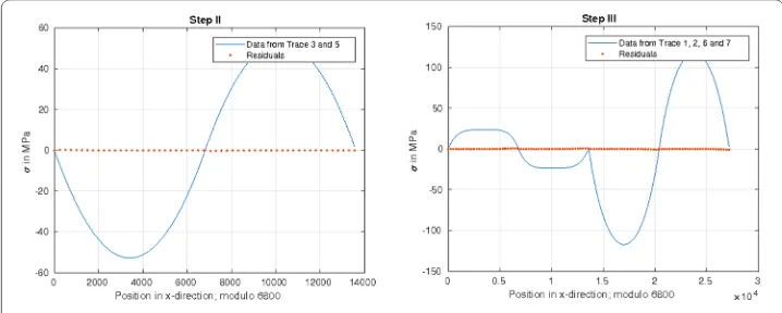
Using the symmetries shown in equations (2) to (8) and known constants from geom-etry the estimation is based on partitioning and sieving the observations in the differ-ent traces, compare Fig.9to 11. This is done in (up to) six steps, for description pur-poses with data generated via finite-element simulation in the description and real data subsequently, with least squares for each local estimation, starting with an initial value θ0= (α0
0, . . . ,α0n1,β00, . . . ,βn20,γ00,γ10,γ20) from mechanics for the internal forcesMy,Mz,Mw,
respectively, the exponent is an index for the estimation step, the coefficientsn1,n2≥0 are the polynomials degrees. Furthermore, we useα,˜ β˜,γ˜to denote the moments’ constants multiplied with the geometry factors to obtain stresses. The procedure works as follows:
Figure 10 Left:Estimation ofMy.Right:Estimation ofMz+Mw
Figure 11 Left:Update of the estimation ofMy.Right:Update of the estimation ofMz+Mwand termination
Algorithm First, normalise all observations, i.e. remove the constantsc= (c1, . . . ,c7), and keep them for estimation of the occurring constantsα0,β0,γ0. The part left is the sum of normal and residual stress. Note, that the separation in residual and normal stress (i.e. splitting the constant) is not possible in general unless further information, e.g. from micro magnetics, see Sect.4.5, are available.
Second, estimate the internal forceMyfrom traces 3 and 5 using (robust) Least Squares
(cf. [20]) under the constraint | ˜α01| ≤ |c3|,|c5|. The estimate obtained is called θ2 = (α2
0, . . . ,αn12 ,β00, . . . ,βn20 ,γ00,γ10,γ20) (analogously without mentioning in the sequel). Third, estimate the internal forces Mz +Mw (note, that they are either both
triv-ial/constant or linearly independent, thus, there is a unique solution to this estimation problem) in traces 1, 2, 3, 5, 6, 7 under knowledge ofMy(i.e. subtraction) from the
previ-ous step and keep the constraints| ˜β03+γ˜03+α˜02| ≤ |c1|,|c2|,|c6|,|c7|.
Fourth, as first update step, estimate the internal forceMyusing the information in all
traces (except trace 4) under knowledge ofMzandMw(i.e. subtraction) from the previous
step (see Fig.10) and keep the constraints| ˜β03+γ˜03+α˜40| ≤ |c1|,|c2|,|c6|,|c7|.
Fifth, as second update step, estimate the internal forcesMz+Mwin traces 1, 2, 6, 7 under
knowledge ofMyfrom the previous step (see Fig.11) and keep the constraints| ˜β05+γ˜05+ ˜
α40| ≤ |c1|,|c2|,|c6|,|c7|.
Figure 12 Example of a contaminated dataset with less points and reasonable result after 36 iterations
random and non-repeating order at mostMtimes, checking the Cauchy criterion after each iteration.
An example with less and contaminated data and bad initial values, including the ne-cessity of the last step, can be seen in the following Fig.12: The trend in the residuals is quite clear: starting point is a quite bad initial value which gets better and better with an increasing number of iterations. This corresponds to two effects in the construction of the estimates: First, we use the least squares approach by Howard and Welsh (compare [20]), which avoids deterioration of the estimate. Second, the ping-pong between differ-ent datasets improves the local estimates, thus, the global ones. Therefore, we can clip the following:
• Weaker dependence structures are crucial for the application of the estimation techniques, therefore, the dependency reduction was necessary.
• The constantsα0,β0,γ0can not be estimated simultaneously in steps 3 and 5, thus, a
fixed-constant approach has to be chosen including several trials.
• A deterioration of the local estimation is not possible due the construction of the Levenberg-Marquardt least squares, cf. [21,22].
• Using the geometry constants from equations (2) to (8) and the estimatesα0,β0,γ0
from the final estimation, the remaining parts ofc,c˜is the estimate for the sum of residual and normal stress and with knowledge of the normal stress, a decomposition in residual and normal stress can be done, see [18].
• An absolute value bound (or in some cases: estimate) for the normal stress could be obtained via
N= min
i=1,...,7ci– (gyi·α0+gzi·β0+gwi·γ0),
an estimate for the residual stresses is given via
Ei=ci±N– (gyi·α0+gzi·β0+gwi·γ0).
Note, that those estimates are not necessarily consistent ones.
uniformly bounded variance0 <σ2<∞.
Then the estimates used in every step are consistent.Furthermore,θ is a consistent esti-mate for the coefficients of the internal forces.
Proof The statement follows mainly from the Theorems 10.3, 20.3 and 24.1 in [23] and
Slutsky’s Lemma.
Theorem 2(Doktor, Stockis) Consider the setup of Theorem1.Then the estimates
ob-tained for the internal forces are asymptotically normally distributed.
Proof The statement for sieve and partition estimates follows from consistency and The-orems 11.4 and 21.1 in [23], the final statement uses additionally the rules of calculus for
the multivariate normal distribution.
Note, that this statement can be generalized in a robust setting according to [17] unless the rate of convergence decreases which is of high importance in practical applications as recording data is time-consuming and might be expansive.
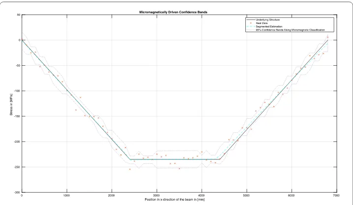
4.5 Further improvement with micromagnetics
The determination of valid confidence bands is a necessity for proper safety concepts in civil engineering. Further, the classification of residuals observed in ultrasonics has to be done properly to avoid economical and ecological disadvantages. Based on [18], additional micromagnetic measurements are used to link techniques and concepts.
4.5.1 Reduction of complexity
The devices used to record micromagnetic quantities measure 42 different quantities. They use four different implemented sensors which are rather expensive. To make the device handable in practice, a goal is the reduction of the number of quantities necessary without significant loss of quality. For this purpose we applied multiple statistical tests of independence, based onχ2-tests, for details, we refer to [15]. With a (combined) level of 10%, 36 quantities are identified to be stochastically dependent. The quantities left are driven by two sensors only: the Barkhausen effect and incremental permeability, which halves the amount of sensors required, see [8] for details.
4.5.2 Combining ultrasonic waves and micromagnetism
Figure 13 The density of the distribution of the residuals estimated using a Gaussian kernel and
measurements is given in blue, the mixture of the densities estimated using the link-function in orange. The difference is minimal due to bias-effects which vanishes asymptotically
Figure 14 The analytic (blue) curve, the under idealised conditions recorded data (orange) the estimated curve (cyan) with confidence bands (purple)
Figure 15 The analytic (blue) curve, the under idealised conditions recorded data (orange) the estimated curve (cyan) with smaller confidence bands (purple) compared to the classical setup
5 Discussion and results
5.1 A simulation example
The estimation technique described inAlgorithmhas been applied to datasets generated via Finite-Element simulation. The example inputs were an IPE 360, length 6800 mm and fork-mounted single-carrier with line load only which reduces the amount of variables to be estimated. The internal forces for the simulation are analytically given as
My= 0 + 56,208.7654·x– 8.2642·x2,
Mz= 0 – 3382.1138·x+ 0.49737·x2,
Mw= 0 + 856.7814·2,179,723.9601· 1 –cosh(x) +tanh
6800 2
·sinh(x)
,
E1= 12,
N= 0
and have minor fluctuations due to the FE-grid. In the sequel, a cross-validation approach for verification is used. Concretely, the stresses in traces 2–7 were used for estimation and the stress in trace 1 (all internal forces occur in trace 1) for verification, compare Fig.6and Eqs. (2)–(8). Thus, the residuals are given by
x=ς1(x) –
z1
iy
ˆ
My(x) +
y1
iz
ˆ
Mz(x) +
q1
iw
ˆ
Mw(εx) +Eˆ1+Nˆ
for known constants from geometry.
For 69 (0 mm, 100 mm, . . . , 6800 mm) equidistant values for the stresses the following estimates are obtained:
ˆ
ˆ
Mz= 0 – 3382.1138·x+ 0.49737·x2,
ˆ
Mw= 856.7814·2,179,723.9599· 1 –cosh(εx) +tanh
6800ε 2
·sinh(εx)
,
ˆ
E1+Nˆ = 12
with residual meanμ= 0.012 and standard deviationσ= 0.16 which is close to the non-equidistant (69 points randomly chosen) case:
ˆ
My= 0 + 56,207.8515·x– 8.264·x2,
ˆ
Mz= 0 – 3382.1142·x+ 0.49737·x2,
ˆ
Mw= 856.7814·2,179,923.3682· 1 –cosh(x) +tanh
6800 2
·sinh(x)
,
ˆ
E1+Nˆ = 12
with residual meanμ= 0.013 and standard deviationσ= 0.18.
A Monte-Carlo study with 1,000,000 independent repetitions leads, for 69 equidistant noisy (additive independent zero-mean normally distributed error terms, standard de-viationσ) stresses, to the following estimated residual means, standard deviations and repetitions of step 6 (upper limit 100 was never reached):
σ 5 10 25 50 75 100
Residual mean –0.089 –0.104 –0.054 0.107 0.224 0.0189
Residual standard deviation 0.821 1.158 2.491 4.848 7.269 9.711
Mean number of iterations 2 5 7 11 15 21
which demonstrates principal applicability of the estimation technique.
5.2 A real data example
Figure 16 The non-scaled initial data. Several outliers due to dramatically missevaluated AScans are obvious and corrected in a preprocessing step before further estimation
Figure 17 The final estimation of the lab tested, coated beam. The classical approach leads to an
unsatisfactory evaluation. Therefore, a robust weight function has been in use too, which improves the results and comes close to the underlying structure
6 Conclusion and further developments
square estimation leads to surprisingly good results, even for small sample sizes. Further-more, these estimation techniques can be further generalised in a future work to a robust setting (e.g. optimally bias robust estimators) to keep applicability for e.g. coated beams. This ends up in new and improved security, usage and sustainability concepts for existing buildings including all relevant internal forces.
Acknowledgements
Special thanks to Claudia Redenbach and Peter Ruckdeschel for several fruitful discussions about mathematics and its implementation. Further, thanks to Claudia Seck and Nicole Schmeckebier for fruitful discussions regarding structural analysis.
Funding
This contribution uses results obtained in the research projectBestandsbewertung von Stahlbauwerken mithilfe
zerstörungsfreier Prüfverfahrensupported by the Forschungsvereinigung Stahlbau in the context of IGF (IGF-Vorhaben 466
ZN) based on a resolution of the German Bundestag as well as the AiF-ZIM-ProjectBestandsbewertung von Stahlbauwerken mithilfe zerstörungsfreier Prüfverfahren, FZ: ZF4163502LT6, by the Federal Ministry of Economic Affairs and Energy.
Abbreviations
Not applicable.
Availability of data and materials
Please contact author for data requests.
Competing interests
The authors declare that they have no competing interests.
Authors’ contributions
The main idea of this paper was proposed by MD and the implementation was also done by MD. JPS supported MD in mathematical modeling as well as in validation. The general engineering context was proposed by WK and CF. CF and WK assisted MD in mechanical modeling and JPS helped preparing the manuscript. All authors read and approved the final manuscript.
Publisher’s Note
Springer Nature remains neutral with regard to jurisdictional claims in published maps and institutional affiliations.
Received: 16 February 2018 Accepted: 8 October 2018
References
1. BeuthVerlag: DIN 1055100: Einwirkungen Auf Tragwerke Teil 100: Grundlagen der Tragwerksplanung -Sicherheitskonzept und Bemessungsregeln. Berlin. 2001-03.
2. Normenausschuss Bauwesen (NABau) im DIN Deutsches Institut für Normung e.V.: DIN 1076: Ingenieurbauwerke Im Zuge Von Straßen und Wegen. Überwachung und Prüfung. Berlin. 1999.
3. Deutsche Bahn AG: Richtline DS 805, Tragsicherheit Bestehender Brückenbauwerke. Berlin. 2002.
4. Boller C, Altpeter I, Dobmann G, Rabung M, Schreiber J, Szielasko K, Tschunky R. Electromagnetism as a means for understanding material mechanics phenomena in magnetic materials. Materialwissenschaft und Werkstofftechnik. 2011;42:269–77.
5. Boller C, Starke P. Enhanced assessment of ageing phenomena in steel structures based on material data and non-destructive testing. Mater Sci Eng Technol. 2016;47:876–86.
6. Schneider E, Bindseil P, Boller C, Kurz W. Stand der entwicklung zur zerstörungsfreien bestimmung der längsspannung in bewehrungsstäben in betonbauwerken. Beton und Stahlbetonbau. 2012;107(4):244–54. 7. Fox C, Doktor M, Schneider E, Kurz W. Beitrag zur bewertung von stahlbauwerken mithilfe zerstörungsfreier
prüfverfahren. Stahlbau. 2016;85(1):1–15.
8. Mayer JP. Aufbau und Kalibrierung Eines Magnetischen Hall-Sensors zur Detektion und Bewertung Von Schädigung an Stahlbauwerken. Seminar project. Institute of Materials Science and Engineering, University of Kaiserslautern; 2016.
9. Kurz W, Fox C, Doktor M, Hanke R, Kopp M, Schwender T, Nüsse G. Bestandsbewertung Von Stahlbauwerken Mithilfe Zerstörungsfreier Prüfverfahren (P 859). Düsseldorf: Forschungsvereinigung Stahlanwendung e.V. (FOSTA); 2016. 10. Kurz W, Fox C. Evaluation of steel buildings by means of non-destructive testing methods. Schriftenreihe des
Studiengangs Bauingenieurwesen der TU Kaiserslautern, Band 18; 2014.
11. Lerman PM. Fitting segmented regression models by grid search. J R Stat Soc, Ser C, Appl Stat. 1980;29(1):77–84. 12. The Mathworks Inc. MATLAB and statistics toolbox release 2017. 2017. Natick: The Mathworks Inc.
13. R Developement Core Team. R: a language and environment for statistical computing. R Foundation for Statistical Computing; 2017.
14. Francke W, Friemann H. Schub und Torsion in Geraden Stäben. Wiesbaden: Vieweg; 2005.
15. Roy SN, Bargmann RE. Tests of multiple independence and the associated confidence bounds. Ann Math Stat. 1958;29(2):491–503.
2010.


![Figure 7 Left: One source of errors is missing one of the echos (compare Abb. 3.7 in [9])](https://thumb-us.123doks.com/thumbv2/123dok_us/9609624.1943232/7.595.117.478.82.205/figure-left-source-errors-missing-echos-compare-abb.webp)