The Thirty-Third AAAI Conference on Artificial Intelligence (AAAI-19)
A Deep Neural Network for Unsupervised Anomaly
Detection and Diagnosis in Multivariate Time Series Data
Chuxu Zhang,
§∗Dongjin Song,
†∗Yuncong Chen,
†Xinyang Feng,
‡∗Cristian Lumezanu,
†Wei Cheng,
†Jingchao Ni,
†Bo Zong,
†Haifeng Chen,
†Nitesh V. Chawla
§§University of Notre Dame, IN 46556, USA †NEC Laboratories America, Inc., NJ 08540, USA
‡Columbia University, NY 10027, USA
§{czhang11,nchawla}@nd.edu,†{dsong,yuncong,lume,weicheng,jni,bzong,haifeng}@nec-labs.com,‡xf2143@columbia.edu
Abstract
Nowadays, multivariate time series data are increasingly col-lected in various real world systems,e.g., power plants, wear-able devices,etc. Anomaly detection and diagnosis in multi-variate time series refer to identifying abnormal status in cer-tain time steps and pinpointing the root causes. Building such a system, however, is challenging since it not only requires to capture the temporal dependency in each time series, but also need encode the inter-correlations between different pairs of time series. In addition, the system should be robust to noise and provide operators with different levels of anomaly scores based upon the severity of different incidents. Despite the fact that a number of unsupervised anomaly detection algorithms have been developed, few of them can jointly address these challenges. In this paper, we propose a Multi-Scale Con-volutional Recurrent Encoder-Decoder (MSCRED), to per-form anomaly detection and diagnosis in multivariate time se-ries data. Specifically, MSCRED first constructs multi-scale (resolution) signature matrices to characterize multiple levels of the system statuses in different time steps. Subsequently, given the signature matrices, a convolutional encoder is em-ployed to encode the inter-sensor (time series) correlations and an attention based Convolutional Long-Short Term Mem-ory (ConvLSTM) network is developed to capture the tempo-ral patterns. Finally, based upon the feature maps which en-code the inter-sensor correlations and temporal information, a convolutional decoder is used to reconstruct the input sig-nature matrices and the residual sigsig-nature matrices are further utilized to detect and diagnose anomalies. Extensive empiri-cal studies based on a synthetic dataset and a real power plant dataset demonstrate that MSCRED can outperform state-of-the-art baseline methods.
Introduction
Complex systems are ubiquitous in modern manufacturing industry and information services. Monitoring the behav-iors of these systems generates a substantial amount of mul-tivariate time series data, such as the readings of the net-worked sensors (e.g., temperature and pressure) distributed in a power plant or the connected components (e.g., CPU us-age and disk I/O) in an Information Technology (IT) system. ∗This work was done when the first and fourth authors were
summer interns at NEC Laboratories America. Dongjin Song is the corresponding author.
Copyright c2019, Association for the Advancement of Artificial Intelligence (www.aaai.org). All rights reserved.
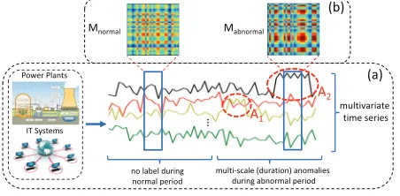
Figure 1: (a) Unsupervised anomaly detection and diagnosis in multivariate time series data. (b) Different system signa-ture matrices between normal and abnormal periods.
A critical task in managing these systems is to detect anoma-lies in certain time steps such that the operators can take fur-ther actions to resolve underlying issues. For instance, an anomaly score can be produced based on the sensor data and it can be used as an indicator of power plant failure (Len, Vittal, and Manimaran 2007). An accurate detection is crucial to avoid serious financial and business losses as it has been reported that 1 minute downtime of an automo-tive manufacturing plant may cost up to20,000US dollars (Djurdjanovic, Lee, and Ni 2003). In addition, pinpointing the root causes,i.e., identifying which sensors (system com-ponents) are causes to an anomaly, can help the system op-erator perform system diagnosis and repair in a timely man-ner. In real world applications, it is common that a short term anomaly caused by temporal turbulence or system sta-tus switch may not eventually lead to a true system failure due to the auto-recovery capability and robustness of mod-ern systems. Therefore, it would be ideal if an anomaly de-tection algorithm can provide operators with different levels of anomaly scores based upon the severity of various inci-dents. For simplicity, we assume that the severity of an in-cident is proportional to the duration of an anomaly in this work. Figure 1(a) illustrates two anomalies,i.e.,A1andA2 marked by red dash circle, in multivariate time series data. The root causes are yellow and black time series, respec-tively. The duration (severity level) ofA2is larger thanA1.
di-agnose anomalies, one main problem is that few or even no anomaly label is available in the historical data, which makes the supervised algorithms (G¨ornitz et al. 2013) infeasible. In the past few years, a substantial amount of unsupervised anomaly detection methods have been developed. The most prominent techniques include dis-tance/clustering methods (He, Xu, and Deng 2003; Hau-tama¨ki, Ka¨rkka¨ınen, and Fra¨nti 2004), probabilistic methods (Chandola, Banerjee, and Kumar 2009), density estimation methods (Manevitz and Yousef 2001), temporal prediction approaches (Chen et al. 2008; G¨unnemann, G¨unnemann, and Faloutsos 2014), and the more recent deep learning techniques (Qin et al. 2017; Zhou and Paffenroth 2017; Wu et al. 2018; Zong et al. 2018). Despite the intrinsic unsu-pervised setting, most of them may still not be able to detect anomalies effectively due to the following reasons:
• There exists temporal dependency in multivariate time se-ries data. Due to this reason, distance/clustering methods,
e.g., k-Nearest Neighbor (kNN) (Hautama¨ki, Ka¨rkka¨ınen, and Fra¨nti 2004)), classification methods,e.g., One-Class SVM (Manevitz and Yousef 2001), and density estima-tion methods, e.g., Deep Autoencoding Gaussian Mix-ture Model (DAGMM) (Zong et al. 2018), may not per-form well since they cannot capture temporal dependen-cies across different time steps.
• Multivariate time series data usually contain noise in real word applications. When the noise becomes relatively se-vere, it may affect the generalization capability of tempo-ral prediction models, e.g., Autoregressive Moving Av-erage (ARMA) (Brockwell and Davis 2013) and LSTM encoder-decoder (Qin et al. 2017), and increase the false positive detections.
• In real world application, it is meaningful to provide oper-ators with different levels of anomaly scores based upon the severity of different incidents. The existing methods for root cause analysis,e.g., Ranking Causal Anomalies (RCA) (Cheng et al. 2016), are sensitive to noise and can-not handle this issue.
In this paper, we propose a Multi-Scale Convolutional Recurrent Encoder-Decoder (MSCRED) to jointly consider the aforementioned issues. Specifically, MSCRED first con-structs multi-scale (resolution) signature matrices to charac-terize multiple levels of the system statuses across different time steps. In particular, different levels of the system sta-tuses are used to indicate the severity of different abnormal incidents. Subsequently, given the signature matrices, a con-volutional encoder is employed to encode the inter-sensor (time series) correlations patterns and an attention based Convolutional Long-Short Term Memory (ConvLSTM) net-work is developed to capture the temporal patterns. Finally, with the feature maps which encode the inter-sensor corre-lations and temporal information, a convolutional decoder is used to reconstruct the signature matrices and the residual signature matrices are further utilized to detect and diagnose anomalies. The intuition is that MSCRED may not recon-struct the signature matrices well if it never observes simi-lar system statuses before. For example, Figure 1(b) shows two signature matricesMnormalandMabnormalduring normal
and abnormal periods. Ideally, MSCRED cannot reconstruct
Mabnormalwell as training matrices (e.g.,Mnormal) are distinct fromMabnormal. To summarize, the main contributions of our work are:
• We formulate the anomaly detection and diagnosis prob-lem as three underlying tasks, i.e., anomaly detection, root cause identification, and anomaly severity (dura-tion) interpretation. Unlike previous studies which inves-tigate each problem independently, we address these is-sues jointly.
• We introduce the concept of system signature matrix, de-velop MSCRED to encode the inter-sensor correlations via a convolutional encoder, incorporate temporal pat-terns with attention based ConvLSTM networks, and re-construct signature matrix via a convolutional decoder. As far as we know, MSCRED is the first model that considers correlations among multivariate time series for anomaly detection and can jointly resolve all the three tasks. • We conduct extensive empirical studies on a synthetic
dataset as well as a power plant dataset. Our results demonstrate the superior performance of MSCRED over state-of-the-art baseline methods.
Related Work
Unsupervised anomaly detection on multivariate time series data is a challenging task and various types of approaches have been developed in the past few years.
One traditional type is the distance methods (Hautama¨ki, Ka¨rkka¨ınen, and Fra¨nti 2004). For instance, the k-Nearest Neighbor (kNN) algorithm (Hautama¨ki, Ka¨rkka¨ınen, and Fra¨nti 2004) computes the anomaly score of each data sam-ple based on the average distance to its k nearest neigh-bors. Similarly, the clustering models (He, Xu, and Deng 2003) cluster different data samples and find anomalies via a predefined outlierness score. In addition, the classification methods,e.g., One-Class SVM (Manevitz and Yousef 2001), models the density distribution of training data and classi-fies new data as normal or abnormal. Although these meth-ods have demonstrated their effectiveness in various appli-cations, they may not work well on multivariate time series since they cannot capture the temporal dependencies appro-priately. To address this issue, temporal prediction methods,
e.g., Autoregressive Moving Average (ARMA) (Brockwell and Davis 2013) and its variants, have been used to model temporal dependency and perform anomaly detection. How-ever, these models are sensitive to noise and thus may in-crease false positive results when noise is severe. Other tra-ditional methods include correlation methods (Kriegel et al. 2012), ensemble methods (Lazarevic and Kumar 2005),etc.
capa-bility than traditional methods. Despite their effectiveness, they cannot jointly consider the temporal dependency, noise resistance, and the interpretation of severity of anomalies.
In addition, our model design is inspired by fully con-volutional neural networks (Long, Shelhamer, and Darrell 2015), convolutional LSTM networks (Shi et al. 2015), and attention technique (Bahdanau, Cho, and Bengio 2014). This paper is also related to other time series applications such as classification (Karim et al. 2018), segmentation (Lemire 2007), and so on.
MSCRED Framework
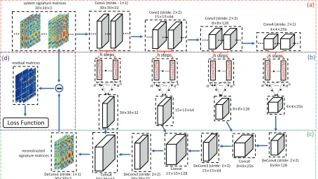
In this section, we first introduce the problem we aim to study and then we elaborate the proposed Multi-Scale Con-volutional Recurrent Encoder-Decoder (MSCRED) in de-tail. Specifically, we first show how to generate multi-scale (resolution) system signature matrices. Then, we encode the spatial information in signature matrices via a convolutional encoder and model the temporal information via an attention based ConvLSTM. Finally, we reconstruct signature matri-ces based upon a convolutional decoder and use a square loss to perform end-to-end learning.
Problem Statement
Given the historical data ofntime series with lengthT,i.e.,
X = (x1,· · ·,xn)T ∈Rn×T, and assuming that there
ex-ists no anomaly in the data, we aim to achieve two goals: • Anomaly detection,i.e., detecting anomaly events at
cer-tain time steps afterT.
• Anomaly diagnosis, i.e., given the detection results, identifying the abnormal time series that are most likely to be the causes of each anomaly and interpreting the anomaly severity (duration scale) qualitatively.
Characterizing Status with Signature Matrices
The previous studies (Hallac et al. 2017; Song et al. 2018) suggest that the correlations between different pairs of time series are critical to characterize the system status. To represent the inter-correlations between different pairs of time series in a multivariate time series segment fromt −w to t, we construct an n×n signature matrix Mt
based upon the pairwise inner-product of two time se-ries within this segment. Two examples of signature ma-trices are shown in Figure 1(b). Specifically, given two time series xw
i = (xti−w, xit−w−1,· · · , xti) and xwj = (xtj−w, xjt−w−1,· · ·, xt
j) in a multivariate time series
seg-mentXw, their correlationmt
ij ∈Mtis calculated with:
mtij =
w
δ=0xti−δxtj−δ
κ (1)
where κ is a rescale factor (κ = w). The signature ma-trix,i.e.,Mt, not only can capture the shape similarities and
value scale correlations between two time series, but also is robust to input noise as the turbulence at certain time series has little impact on the signature matrices. In this work, the interval between two segments is set as 10. In addition, to characterize system status at different scales, we constructs
(s= 3) signature matrices with different lengths (w= 10, 30, 60) at each time step.
Convolutional Encoder
We employ a fully convolutional encoder (Long, Shelhamer, and Darrell 2015) to encode the spatial patterns of system signature matrices. Specifically, we concatenateMtat
dif-ferent scales as a tensorXt,0∈Rn×n×s, and then feed it to
a number of convolutional layers. Assuming thatXt,l−1 ∈ Rnl−1×nl−1×dl−1 denotes the feature maps in the (l−1)-th layer, the output ofl-th layer is given by:
Xt,l=f(Wl∗ Xt,l−1+bl) (2)
where∗denotes the convolutional operation,f(·)is the ac-tivation function,Wl ∈Rkl×kl×dl−1×dl denotesd
l
convo-lutional kernels of size kl×kl×dl−1,bl ∈ Rdl is a bias
term, andXt,l∈Rnl×nl×dldenotes the output feature map
atl-th layer. In this work, we use Scaled Exponential Linear Unit (SELU) as the activation function and 4 convolutional layers,i.e., Conv1-Conv4 with 32 kernels of size3×3×3, 64 kernels of size3×3×32, 128 kernels of size2×2×64, and 256 kernels of size2×2×128, as well as1×1,2×2,
2×2, and2×2strides, respectively. Note that the exact order of the time series based on which the signature matrices are formed is not important, because for any given permutation, the resulting local patterns can be captured by the convolu-tional encoder. Figure 2(a) illustrates the detailed encoding process of signature matrices.
Attention based ConvLSTM
The spatial feature maps generated by convolutional encoder is temporally dependent on previous time steps. Although ConvLSTM (Shi et al. 2015) has been developed to cap-ture the temporal information in a video sequence, its perfor-mance may deteriorate as the length of sequence increases. To address this issue, we develop an attention based ConvL-STM which can adaptively select relevant hidden states (fea-ture maps) across different time steps. Specifically, given the feature mapsXt,lfrom thel-th convolutional layer and
pre-vious hidden stateHt−1,l ∈ Rnl×nl×dl, the current hidden
stateHt,lis updated withHt,l=ConvLSTM(Xt,l,Ht−1,l),
where the ConvLSTM cell (Shi et al. 2015) is formulated as:
zt,l=σ( ˜Wl
X Z∗ Xt,l+ ˜WHZl ∗ Ht−1,l+ ˜WCZk ◦ Ct−1,l+ ˜blZ)
rt,l=σ( ˜WX Rl ∗ Xt,l+ ˜WHRl ∗ Ht−1,l+ ˜WCRl ◦ Ct−1,l+ ˜blR)
Ct,l=zt,l◦tanh( ˜Wl
X C∗ Xt,l+ ˜WHCl ∗ Ht−1,l+ ˜blC)+
rt,l◦ Ct−1,l
ot,l=σ( ˜Wl
X O∗ Xt,l+ ˜WHO∗ Ht−1,l+ ˜WCO◦ Ct,l+ ˜blO)
Ht,l=ot,l◦tanh(Ct,l)
(3)
where ∗ denotes the convolutional operator, ◦
repre-sents Hadamard product, σ is the sigmoid function,
˜ Wl
X Z,W˜HZl ,W˜CZl ,W˜X Rl ,W˜HRl ,W˜CRl ,W˜X Cl ,W˜HCl ,W˜X Ol ,
˜ Wl
HO,W˜COl ∈ Rk˜l×k˜l×d˜l×d˜l are d˜l convolutional kernels
of size k˜l ×k˜l ×d˜l and ˜blZ,b˜lR,˜blC,˜blO ∈ Rd˜l are bias
"
#
&% $
%
%
$
#
"
$#
Figure 2: Framework of the proposed model: (a) Signature matrices encoding via fully convolutional neural networks. (b) Tem-poral patterns modeling by attention based convolutional LSTM networks. (c) Signature matrices decoding via deconvolutional neural networks. (d) Loss function.
maintain the same convolutional kernel size as convolu-tional encoder at each layer. Note that all the input Xt,l, cell outputsCt,l, hidden statesHt−1,l, and gateszt,l,rt,l,
ot,lare 3D tensors, which is different from LSTM. We tune step lengthh(i.e.,the number of previous segments) and set it as 5 due to the best empirical performance. In addition, considering not all previous steps are equally correlated to the current state Ht,l, we adopt a temporal attention mechanism to adaptively select the steps that are relevant to current step and aggregate the representations of those informative feature maps to form a refined output of feature mapsHˆt,l, which is given by:
ˆ
Ht,l=
i∈(t−h,t)
αiHi,l, αi= exp{
Vec(Ht,l)TVec(Hi,l)
χ }
i∈(t−h,t)exp{Vec(H
t,l)TVec(Hi,l)
χ } (4) where Vec(·)denotes vector andχis a rescale factor (χ= 5.0). That is, we take the last hidden stateHt,las the group level context vector and measure the importance weightsαi of previous steps through a softmax function. Unlike the general attention mechanism (Bahdanau, Cho, and Bengio 2014) that introduces transformation and context parame-ters, the above formulation is purely based on the learned hidden feature maps and achieves the similar function as the former. Essentially, the attention based ConvLSTM jointly models the spatial patterns of signature matrices with tem-poral information at each convolutional layer. Figure 2(b) illustrates the temporal modeling procedure.
Convolutional Decoder
To decode the feature maps obtained in previous step and get the reconstructed signature matrices, we design a convo-lutional decoder which is formulated as:
ˆ
Xt,l−1= f( ˆWt,lHˆt,l+ ˆbt,l), l= 4 f( ˆWt,l[ ˆHt,l⊕Xˆt,l] + ˆbt,l), l= 3,2,1 (5)
detection performance, as we will demonstrate in the exper-iment. Figure 2(c) illustrates the decoding procedure.
Loss Function
For MSCRED, the objective is defined as the reconstruction errors over the signature matrices,i.e.,
LM SCRED =
t s
c=1
Xt,0
:,:,c−Xˆ:t,,:0,c
2
F (6)
where Xt,0
:,:,c ∈ Rn×n. We employ mini-batch stochastic
gradient descent method together with the Adam optimizer (Kingma and Ba 2014) to minimize the above loss. After sufficient number of training epochs, the learned neural net-work parameters are utilized to infer the reconstructed signa-ture matrices of validation and test data. Finally, we perform anomaly detection and diagnosis based on the residual sig-nature matrices, which will be elaborated in the next section.
Experiments
In this section, we conduct extensive experiments to answer the following research questions:
• Anomaly detection.Whether MSCRED can outperform baseline methods for anomaly detection in multivariate time series (RQ1)? How does each component of MS-CRED affect its performance (RQ2)?
• Anomaly diagnosis. Whether MSCRED can perform root cause identification (RQ3) and anomaly severity (du-ration) interpretation (RQ4) effectively?
• Robustness to noise.Compared with baseline methods, whether MSCRED is more robust to input noise (RQ5)?
Experimental Setup
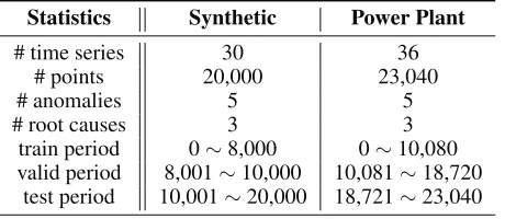
Data. We use a synthetic dataset and a real world power plant dataset for empirical studies. The detailed statistics and settings of these two datasets are shown in Table 1.
(Synthetic data) Each time series is formulated as:
S(t) =
⎧ ⎪ ⎪ ⎨ ⎪ ⎪ ⎩
sin
C1
[(t−t0)/ω]
C2
+λ·
C3
, srand= 0
cos
C1
[(t−t0)/ω]
C2
+λ·
C3
, srand= 1 (7)
wheresrandis a 0 or 1 random seed. The above formula cap-tures three attributes of multivariate time series: (a) trigono-metric function (C1) simulates temporal patterns; (b) time delayt0 ∈ [50,100]and frequencyω ∈ [40,50](C2) sim-ulates various periodic cycles; (c) random Gaussian noise
∼ N(0,1)scaled by factorλ = 0.3 (C3) simulates data noise as well as various shapes. In addition, two sinusoidal waves have high correlation if their frequencies are sim-ilar and they are almost in-phase. By randomly selecting frequency and phase of each time series, we expect some pairs to have high correlations while some have low corre-lations. We randomly generate 30 time series and each in-cludes 20000 points. Besides, 5 shock wave like anomalies (with similar value range of normal data, as the examples in
Table 1: The detailed statistics and settings of two datasets. Statistics Synthetic Power Plant
# time series 30 36
# points 20,000 23,040
# anomalies 5 5
# root causes 3 3
train period 0∼8,000 0∼10,080
valid period 8,001∼10,000 10,081∼18,720
test period 10,001∼20,000 18,721∼23,040
Figure 1(a)) are randomly injected into 3 random time se-ries (root causes) during test period. The duration of each anomaly belongs to one of the three scales,i.e., 30, 60, 90.
(Power plant data) This dataset was collected on a real power plant. It contains 36 time series generated by sensors distributed in the power plant system. It has 23,040 time steps and contains one anomaly identified by the system op-erator. Besides, we randomly inject 4 additional anomalies (similar to what we did in the synthetic data) into the test period for thorough evaluation.
Baseline methods. We compare MSCRED with eight baseline methods of four categories, i.e., classification model, density estimation model, temporal prediction model, and variants of MSCRED.
• Classification model. It learns a decision function and classifies test data as similar or dissimilar to the training set. We use One-Class SVM model (OC-SVM) (Manevitz and Yousef 2001) for comparison.
• Density estimation model. It models data density for outlier detection. We use Deep Autoencoding Gaussian Mixture model (DAGMM) (Zong et al. 2018) and take the energy score (Zong et al. 2018) as the anomaly score. • Prediction model. It models the temporal dependen-cies of training data and predicts the value of test data. We employ three methods: History Average (HA), Auto-Regression Moving Average (ARMA) (Brockwell and Davis 2013) and LSTM encoder-decoder (LSTM-ED) (Bahdanau, Cho, and Bengio 2014). The anomaly score is defined as the average prediction error over all time se-ries.
• MSCRED variants.Besides the above baseline methods, we consider three variants of MSCRED to justify the ef-fectiveness of each component: (1) CNNEDConvLSTM(4) is MS-CRED with attention module and first three ConvLSTM layers been removed. (2) CNNEDConvLSTM(3,4) is MSCRED with attention module and first two ConvLSTM layers been removed. (3) CNNEDConvLSTM is MSCRED with attention module been removed.
In other words, the number of elements whose value is larger than a given threshold θin the residual signature matrices andθis detemined empirically over different datasets.
Evaluation metrics. We use three metrics,i.e.,Precision, Recall, and F1 Score, to evaluate the anomaly detection performance of each method. To detect anomaly, we fol-low the suggestion of a domain expert by setting a thresh-oldτ =β·max{s(t)valid}, wheres(t)validare the anomaly scores over the validation period andβ ∈[1,2]is set to max-imize the F1 Score over the validation period. Recall and Precision scores over the test period are computed based on this threshold. Experiments on both datasets are repeated 5 times and the average results are reported for comparison. Note that the output of MSCRED contains three channel of residual signature matricesw.r.t.different segment lengths. We use the smallest one (w= 10) for the following anomaly detection and root cause identification evaluation. The per-formance comparison of three channel results will also be provided for anomaly severity interpretation.
Performance Evaluation
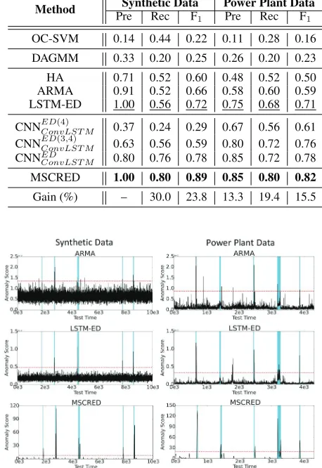
Anomaly detection result (RQ1, RQ2). The performance of different methods for anomaly detection are reported in Table 2, where the best scores are highlighted in bold-face and the best baseline scores are indicated by underline. The last row reports the improvement (%) of MSCRED over the best baseline method.
(RQ1: comparison with baselines)In Table 2, we ob-serve that (a) temporal prediction models perform better than classification and density estimation models, indicat-ing both datasets have temporal dependency; (b) LSTM-ED has better performance than ARMA, showing deep learn-ing model can capture more complex relationship in the data than traditional method; (c) MSCRED performs best on all settings. The improvements over the best baseline range from 13.3% to 30.0%. In other words, MSCRED is much better than baseline methods as it can model both inter-sensor correlations and temporal patterns of multivari-ate time series effectively.
In order to show the comparison in detail, Figure 3 pro-vides case study of MSCRED and two best baseline meth-ods,i.e., ARMA and LSTM-ED, for both datasets. We can observe that the anomaly score of ARMA is not stable and the results contain many false positives and false negatives. Meanwhile, the anomaly score of LSTM-ED is smoother than ARMA while still contains several false positives and false negatives. MSCRED can detect all anomalies without any false positive and false negative.
To demonstrate a more convincing evaluation, we do ex-periment on another synthetic data with 10 anomalies (it is easy to generate larger data with more anomalies). The av-erage recall and precision scores (5 repeated experiments) of MSCRED are (0.84, 0.95) while the values of LSTM-ED are (0.64, 0.87). In addition, we do experiment on another large power plant data which has 920 sensors and 11 labeled anomalies. The recall and precision scores of MSCRED are (7/11, 7/13) while the values of LSTM-ED are (5/11, 5/17). All evaluation results show the effectiveness of our model.
Table 2: Anomaly detection results on two datasets.
Method Synthetic Data Power Plant Data
Pre Rec F1 Pre Rec F1
OC-SVM 0.14 0.44 0.22 0.11 0.28 0.16
DAGMM 0.33 0.20 0.25 0.26 0.20 0.23
HA 0.71 0.52 0.60 0.48 0.52 0.50
ARMA 0.91 0.52 0.66 0.58 0.60 0.59
LSTM-ED 1.00 0.56 0.72 0.75 0.68 0.71
CNNEDConvLST M(4) 0.37 0.24 0.29 0.67 0.56 0.61 CNNEDConvLST M(3,4) 0.63 0.56 0.59 0.80 0.72 0.76 CNNED
ConvLST M 0.80 0.76 0.78 0.85 0.72 0.78
MSCRED 1.00 0.80 0.89 0.85 0.80 0.82
Gain (%) – 30.0 23.8 13.3 19.4 15.5
Figure 3: Case study of anomaly detection. The shaded re-gions represent anomaly periods. The red dash line is the cutting threshold of anomaly.
(RQ2: comparison with model variants)In Table 2, we also observe that by increasing the number of ConvLSTM layers, the performance of MSCRED improves. Specifically,
CNNED
ConvLSTM outperforms CNN ED(3,4)
ConvLSTM and the perfor-mance of CNNEDConvLSTM(3,4) is superior than CNNEDConvLSTM(4) , in-dicating the effectiveness of ConvLSTM layers and stacked decoding process for model refinement. We also observe that
CNNED
ConvLSTM is worse than MSCRED, suggesting that at-tention based ConvLSTM can further improve anomaly de-tection performance.
Figure 4: Average distribution of attention weights at the last two ConvLSTM layers in the power plant data.
Figure 5: Performance of root cause identification.
than the current timestep (step 5), are assigned lower weights than in the distribution for normal segments. In other words, the attention modules show high sensitivity to system status change and thus is beneficial for anomaly detection.
Root cause identification result (RQ3). As one of the anomaly diagnosis tasks, root cause identification depends on good anomaly detection performance. Therefore, we compare the performances of MSCRED and the best base-line,i.e., LSTM-ED. Specifically, for LSTM-ED, we use the prediction error of each time series to represent its anomaly score of this series. The same value of MSCRED is defined as the number of poorly reconstructed pairwise correlations in a specific row/column of residual signature matrices as each row/column denotes a time series. For each anomaly event, we rank all time series by their anomaly scores and identify the top-kseries as the root causes. Figure 5 shows the average recall@k(k= 3) in 5 repeated experiments. MS-CRED outperforms LSTM-ED by a margin of 25.9% and
Figure 6: Performance of three channels of MSCRED over different types of anomalies.
Figure 7: Case study of anomaly diagnosis.
32.4% in the synthetic and power plant data, respectively.
Anomaly severity (duration) interpretation (RQ4). The signature matrices of MSCRED include schannels (s= 3 in current experiments) that capture system status at dif-ferent scales. To interpret anomaly severity, we first com-pute different anomaly scores based on the residual signa-ture matrices of three channels, i.e., small, medium, and large with segment size w = 10, 30, and 60, respectively, and denote them as MSCRED(S), MSCRED(M), and MS-CRED(L). Then, we independently evaluate their perfor-mances on three types of anomalies, i.e., short, medium, and long with the duration of 10, 30, and 60, respectively. The average recall scores over 5 repeated experiments on two datasets are reported in Figure 6. We can observe that MSCRED(S) is able to detect all types of anomalies and MSCRED(M) can detect both medium and long duration anomalies. On the contrary, MSCRED(L) can only detect the long duration anomaly. Accordingly, we can interpret the anomaly severity by jointly considering the three anomaly scores. The anomaly is more likely to be long duration if it can be detected in all three channels. Otherwise, it may be a short or medium duration anomaly. To better show the effectiveness of MSCRED, Figure 7 provides a case study of anomaly diagnosis in power plant data. In this case, MSCRED(S) detects all of 5 anomalies including 3 short, 1 medium and 1 long duration anomalies. MSCRED(M) misses two short duration anomalies and MSCRED(L) only detects the long duration anomaly. Moreover, four resid-ual signature matrices of injected anomaly events show the
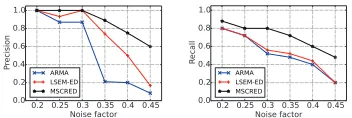
Figure 8: Impact of data noise on anomaly detection.
root causes identification results. We can accurately pinpoint more than half of the anomaly root causes (rows/columns highlighted by red rectangles) in this case.
Robustness to Noise (RQ5). The multivariate time se-ries often contains noise in real world applications, thus it is important for an anomaly detection algorithm to be ro-bust to input noise. To study the roro-bustness of MSCRED for anomaly detection, we conduct experiments in different synthetic datasets by adding various noise factorsλin Equa-tion 7. Figure 8 shows the impact ofλon the performance of MSCRED, ARMA, and LSTM-ED. Similar to previous evaluation, we compute Precision and Recall scores based on the optimized cutting threshold and the average values of 5 repeated experiments are reported for comparison. We can observe that MSCRED consistently outperforms ARMA and LSTM-ED when the scale of noise varies from 0.2 to 0.45. This suggests that, compared with ARMA and LSTM-ED, MSCRED is more robust to the input noise.
Conclusion
In this paper, we formulated anomaly detection and diagno-sis problem, and developed an innovative model,i.e., MS-CRED, to solve it. MSCRED employs multi-scale (resolu-tion) system signature matrices to characterize the whole system statuses at different time segments and adopts a deep encoder-decoder framework to generate reconstructed sig-nature matrices. The framework is able to model both inter-sensor correlations and temporal dependencies of multivari-ate time series. The residual signature matrices are further utilized to detect and diagnose anomalies. Extensive empir-ical studies on a synthetic dataset as well as a power plant dataset demonstrated that MSCRED can outperform state-of-the-art baseline methods.
Acknowledgments
Chuxu Zhang and Nitesh V. Chawla are supported by the Army Research Laboratory under Cooperative Agree-ment Number W911NF-09-2-0053 and the National Science Foundation (NSF) grant IIS-1447795.
References
Bahdanau, D.; Cho, K.; and Bengio, Y. 2014. Neural machine translation by jointly learning to align and translate. InICLR. Brockwell, P. J., and Davis, R. A. 2013. Time series: theory and methods. Springer Science & Business Media.
Chandola, V.; Banerjee, A.; and Kumar, V. 2009. Anomaly detec-tion: A survey.ACM Comput. Surv.41(3):15.
Chen, H.; Cheng, H.; Jiang, G.; and Yoshihira, K. 2008. Exploit-ing local and global invariants for the management of large scale information systems. InICDM, 113–122.
Cheng, W.; Zhang, K.; Chen, H.; Jiang, G.; Chen, Z.; and Wang, W. 2016. Ranking causal anomalies via temporal and dynamical analysis on vanishing correlations. InKDD, 805–814.
Djurdjanovic, D.; Lee, J.; and Ni, J. 2003. Watchdog agent— an infotronics-based prognostics approach for product performance degradation assessment and prediction. Adv. Eng. Inform. 17(3-4):109–125.
G¨ornitz, N.; Kloft, M.; Rieck, K.; and Brefeld, U. 2013. Toward supervised anomaly detection.J. Artif. Intell. Res.46:235–262. G¨unnemann, N.; G¨unnemann, S.; and Faloutsos, C. 2014. Ro-bust multivariate autoregression for anomaly detection in dynamic product ratings. InWWW, 361–372.
Hallac, D.; Vare, S.; Boyd, S.; and Leskovec, J. 2017. Toeplitz inverse covariance-based clustering of multivariate time series data. InKDD, 215–223.
Hautama¨ki, V.; Ka¨rkka¨ınen, I.; and Fra¨nti, P. 2004. Outlier detec-tion using k-nearest neighbour graph. InICPR, 430–433. He, Z.; Xu, X.; and Deng, S. 2003. Discovering cluster-based local outliers.Pattern Recognit. Lett.24(9-10):1641–1650.
Karim, F.; Majumdar, S.; Darabi, H.; and Chen, S. 2018. Lstm fully convolutional networks for time series classification. IEEE Access6:1662–1669.
Kingma, D. P., and Ba, J. 2014. Adam: A method for stochastic optimization.arXiv preprint arXiv:1412.6980.
Kriegel, H.-P.; Kroger, P.; Schubert, E.; and Zimek, A. 2012. Out-lier detection in arbitrarily oriented subspaces. InICDM, 379–388. Lazarevic, A., and Kumar, V. 2005. Feature bagging for outlier detection. InKDD, 157–166.
Lemire, D. 2007. A better alternative to piecewise linear time series segmentation. InSDM, 545–550.
Len, R. A.; Vittal, V.; and Manimaran, G. 2007. Application of sen-sor network for secure electric energy infrastructure. IEEE Trans. Power Del.22(2):1021–1028.
Long, J.; Shelhamer, E.; and Darrell, T. 2015. Fully convolutional networks for semantic segmentation. InCVPR, 3431–3440. Manevitz, L. M., and Yousef, M. 2001. One-class svms for docu-ment classification.J. Mach. Learn. Res.2(Dec):139–154. Qin, Y.; Song, D.; Chen, H.; Cheng, W.; Jiang, G.; and Cottrell, G. 2017. A dual-stage attention-based recurrent neural network for time series prediction. InIJCAI.
Shi, X.; Chen, Z.; Wang, H.; Yeung, D.-Y.; Wong, W.-K.; and Woo, W.-c. 2015. Convolutional lstm network: A machine learning ap-proach for precipitation nowcasting. InNIPS, 802–810.
Song, D.; Xia, N.; Cheng, W.; Chen, H.; and Tao, D. 2018. Deep r-th root of rank supervised joint binary embedding for multivariate time series retrieval. InKDD, 2229–2238.
Wu, X.; Shi, B.; Dong, Y.; Huang, C.; Faust, L.; and Chawla, N. V. 2018. Restful: Resolution-aware forecasting of behavioral time se-ries data. InCIKM, 1073–1082.
Zhou, C., and Paffenroth, R. C. 2017. Anomaly detection with robust deep autoencoders. InKDD, 665–674.