Modelling and analysis of the dynamics
of adaptive temporal–causal network models
for evolving social interactions
Jan Treur
*Background
Network-Oriented Modelling has been proposed as a modelling perspective suitable for processes that are highly dynamic, circular and interactive; e.g. [1, 2]. In different application areas, this modelling perspective has been proposed in different forms: in the contexts of modelling organisations and social systems (e.g. [3–5]), of modelling metabolic processes (e.g. [6]), and of modelling electromagnetic systems (e.g. [7–9]. To address dynamics well, Network-Oriented Modelling based on adaptive temporal–causal networks has been developed [1, 2, 10]. This approach incorporates a continuous (real) time dimension. Adaptive temporal–causal network models are dynamic in two ways: their states change over time based on the causal relations in the network, but these causal relations may also change over time. As, in such networks many interrelating cycles often occur, their emerging behaviour patterns are not always easy to predict or analyse. This may make it hard to evaluate whether observed outcomes of simulations are plausible or might be due to implementation errors.
However, some specific types of properties can also be analysed by calculations in a math-ematical manner, without performing simulations; see, for example [11–16]. Such proper-ties that are found in an analytical mathematical manner can be used for verification of the
Abstract
Background: Network-Oriented Modelling based on adaptive temporal–causal net-works provides a unified approach to model and analyse dynamics and adaptivity of various processes, including mental and social interaction processes.
Methods: Adaptive temporal–causal network models are based on causal relations by which the states in the network change over time, and these causal relations are adap-tive in the sense that they themselves also change over time.
Results: It is discussed how modelling and analysis of the dynamics of the behaviour of these adaptive network models can be performed. The approach is illustrated for adaptive network models describing social interaction.
Conclusions: In particular, the homophily principle and the ‘more becomes more’ principles for social interactions are addressed. It is shown how the chosen Network-Oriented Modelling method provides a basis to model and analyse these social phenomena.
Open Access
© The Author(s) 2017. This article is distributed under the terms of the Creative Commons Attribution 4.0 International License (http://creativecommons.org/licenses/by/4.0/), which permits unrestricted use, distribution, and reproduction in any medium, provided you give appropriate credit to the original author(s) and the source, provide a link to the Creative Commons license, and indicate if changes were made.
RESEARCH
model by checking them for the values observed in simulation experiments. If one of these properties is not fulfilled (and the mathematical analysis was done in a correct manner), then there will be some error in the implementation of the model. In this paper, methods to ana-lyse such properties of temporal–causal network models will be described. They will be illus-trated for two types for dynamic connection weights in adaptive temporal–causal network models modelling evolving social interaction: one based on the homophily principle (“ Mod-elling evolving social interactions by adaptive networks based on the homophily principle” section), and one based on the more becomes more principle (“Modelling evolving social interactions by adaptive networks based on the ‘more becomes more’ principle” section). A preliminary, shorter presentation of part of the work described here can be found in [17].
Network‑Oriented Modelling by temporal–causal networks
The Network-Oriented Modelling approach based on temporal–causal networks, described in more detail in [1, 10] is a generic and declarative dynamic modelling approach based on networks of causal relations. Dynamics is addressed by incorporating a continuous time dimension. This temporal dimension enables modelling by networks that inherently con-tain cycles, such as networks modelling mental or brain processes, or social interaction pro-cesses, and also enables to address the timing of the processes in a differentiated manner. The modelling perspective can incorporate ingredients from different modelling approaches: for example, ingredients that are sometimes used in neural network models, and ingredients that are sometimes used in probabilistic or possibilistic modelling. It is more generic than such methods in the sense that a much wider variety of modelling elements are provided, enabling the modelling of many types of dynamical systems, as described in [1, 10]. The Network-Oriented Modelling approach is supported by a few modelling environments (in Matlab, or in Python, for example) that can be used to model conceptually in a declarative manner, with-out the need of programming. This code is in principle structure-preserving and follows the concepts described in the conceptual description presented in “Conceptual representations of temporal–causal network models” section below. It calculates simulation traces numeri-cally based on the formulae discussed in “From a conceptual representation to a numerical representation” section, and in particular by means of the difference equations. A number of options for often-used combination functions are available within this software and can just be selected. However, for large-scale networks also, dedicated implementations can be developed directly using more efficient programming languages, or dedicated, optimised dif-ferential equation solvers developed to handle large systems of difdif-ferential equations.
Conceptual representations of temporal–causal network models
Temporal–causal network models can be represented at two levels: by a conceptual represen-tation and by a numerical representation. A conceptual representation of a temporal–causal network model can have a (labelled) graphical form (or an equivalent matrix form), as shown in the examples presented below. The following three elements define temporal–causal net-works, and are part of a conceptual representation of a temporal–causal network model:
• connection weight ωX,Y Each connection from a state X to a state Y has a connection weightωX,Y representing the strength of the connection, often between 0 and 1, but
• combination function cY(..) For each state Y (a reference to) a combination function cY(..) is chosen to aggregate the causal impacts of other states on state Y. This can
be a standard function from a library (e.g. a scaled sum function) or an own-defined function.
• speed factor ηY For each state Y, a speed factorηY is used to represent how fast a
state is changing upon causal impact, usually in the [0, 1] interval.
In the first place, a conceptual representation of a temporal–causal network model involves representing in a declarative manner states and connections between them. The connections represent (causal) impacts of states on each other, as assumed to hold for the application domain addressed. Each state X is assumed to have an (activation) level that varies over time, indicated in the numerical representation by a real number X(t). In real-ity, not all causal relations are equally strong, so some notion of strength of a connection from a state X to a state Y is used: a connection weight ωX,Y. Combination functions can have different forms. The applicability of a specific combination rule may depend much on the type of application addressed, and even on the type of states within an application. Therefore, for the Network-Oriented Modelling approach based on temporal–causal net-works a number of standard combination functions are available as options and a number of relevant properties of such combination functions have been identified; e.g. see [10], Table 10, or [1], Chapter 2, Table 2.10. Some of these standard combination functions are scaled sum, product, complementary product, max, min, and simple and advanced logistic sum functions (for some of these examples of combination functions the numerical repre-sentations are discussed in “From a conceptual representation to a numerical representa-tion” section). These options cover elements from different existing approaches, varying from approaches considered for reasoning with uncertainty, probability, possibility or vagueness, to approaches based on neural networks; e.g. [18–26]. In addition, there is still the option to specify any other (non-standard) combination function.
Conceptual representations for an adaptive network
The above three concepts (connection weight, combination function, speed factor) can be considered as parameters representing characteristics in a network model. In a non-adaptive network model, these parameters are fixed over time. But to model processes by adaptive networks, not only the state levels, but also these parameters can change over time. For example, the connection weights can change over time to model evolving connections in network models. For modelling processes as adaptive networks, some of the parameters (such as connection weights) are handled in a similar manner as states. For example, see Fig. 1, where the states affect the connection between them, as hap-pens, for example, in adaptive social networks based on the homophily principle (see “Modelling evolving social interactions by adaptive networks based on the homophily principle” section).
This can be represented differently by considering the connection weight ωX,Y as a
state X,Y that changes over time, represented by an extra node in the network. As a first
step, this node for the state X,Y representing ωX,Y is added and connected; see Fig. 2
for a conceptual representation. In the new situation depicted in Fig. 2, the weight ωX,Y
weight values ωX,Y(t) in the old situation for each t: �X,Y(t)=ωX,Y(t). This state X,Y is affected by both X and Y, so connections from these states to X,Y are incorporated.
Moreover, a connection from X,Y to Y is used to represent the effect of the connection strength on Y, and a connection from X,Y to itself for persistence. The weights of all
these connections are assumed 1; see Fig. 2. As a next step, it is explored what combina-tion funccombina-tions are needed for X,Y and Y in this new situation depicted in Fig. 2.
First, a combination function cX,Y(..) for the state X,Y has to be assumed, to aggregate the impacts of X and Y, and X,Y on X,Y. This will depend on the adaptation principle that is chosen. Next, the new combination function for Y has to be determined. Below the corresponding combination functions will be discussed in more numerical detail.
From a conceptual representation to a numerical representation
Based on a conceptual representation of a temporal–causal network model, in order to obtain a numerical representation of the network model the following concepts can be defined:
• Theimpactof stateXon stateY at timet impactX,Y(t) The impact of state X on state Y at time t is defined by
impactX,Y(t)=ωX,YX(t).
ωX,Y
X Y
Z ωZ,Y
Fig. 1 Conceptual representation of an example with an adaptive connection weight
ω
Z,YΩX,Y
Z 1
1 1 1
1
X Y
Here X(t) is the activation level of state X at t. Note that also a connection from a state Y to itself is allowed. The weight ωY,Y of such a connection can, for example, be
used to model persistence of state Y.
• Theaggregated impacton stateY at timet aggimpactY(t)
When more than one causal relation affects a given state Y, these causal effects have to be combined. To this end, some way to aggregate multiple causal impacts on a state is used; this is done using a combination functioncY(..) that uses the impacts impactXi,Y(t) from states X1, …, Xk on Y as input and provides one aggregated impact value out of them:
• Moreover, not every state has the same extent of flexibility in responding to impact; some states respond fast, and other states may be more rigid and may respond more slowly. Therefore, a speed factorηY of a state Y is used for timing of effectuation of
causal impacts, as shown in the following difference and differential equations:
Given the above concepts, a conceptual representation of a temporal–causal net-work model can be transformed in a systematic and automated manner into a numeri-cal representation of the model, thus obtaining the following difference and differential equation for each state Y, expressed using the basic elements ωX,Y,cY(. . .), and ηY of a
conceptual representation of the model:
The numerical representations of some example combination functions are as follows:.
Numerical representation of a scaled sum combination function
In some cases, it is useful to apply a scaling factor to the sum combination function by dividing it by some scaling factor:
In cases where this combination function is used for a state Y with X1,. . .,Xk con-nected to Y, then this function works as follows on the Xi:
Numerical representation of a simple logistic sum combination function
The logistic sum combination function has two closely related variants, the simple variant and the more advanced variant (see below). In these functions, τ is a threshold parameter and σ a steepness parameter. The simple logistic function is defined as:
aggimpactY(t)=cY(impactX1,Y(t),. . .,impactXk,Y(t)).
Y(t+�t)=Y(t)+ηYaggimpact
Y(t)−Y(t)
�t
dY(t)/dt=η Y
aggimpactY(t)−Y(t) .
Y(t+�t)=Y(t)+η Y
cYωX1,YX1(t),. . .,ωX
k,YXk(t)
−Y(t)
�t
dY(t)/dt=ηYcYωX1,YX1(t),. . .,ωX
k,YXk(t)
−Y(t).
c(V1,. . .,Vk)=ssum(V1,. . .,Vk)=(V1+ · · · +Vk)/.
ssum(ωX
1,YX1,. . .,ωXk,YXk)=(ωX1,YX1+. . .+ωXk,YXk)/.
c(V1,. . .,Vk)=slogistic(V1,. . .,Vk)=
1
To indicate the dependence of σ and τ, sometimes these are used as subscripts: slogisticσ,τ(V1,. . .,Vk).
In cases where this combination function is used for a state Y with X1,. . .,Xk con-nected to Y, then this function works as follows on the Xi:
Numerical representation of an advanced logistic sum combination function
In the simple logistic variant, it holds slogistic(0,. . ., 0)=1/(1+eσ τ), and this is nonzero, which is undesirable property as it creates in an unintended manner activation out of no activation. This issue is compensated for in the advanced variant. The advanced logistic sum combination function is defined as
To indicate the dependence of σ and τ, sometimes these are used as subscripts:
For an overview of a number of standard combination functions, see Table 1.
Numerical representations for an adaptive network
In the simple example depicted in Fig. 1, Y has another impact from Z, besides the impact from X. Then in the new situation depicted in Fig. 2, there are not just two but three states with impact on Y, namely X, Z and X,Y. This requires a new combination function
c∗Y(V1,V2,W) for Y with three arguments, which is applied to the impacts X(t),ωZ,XZ(t)
and �X,Y(t) on Y, obtaining aggregated impact c∗Y(X(t),ωZ,XZ(t),�X,Y(t)). This aggre-gated impact is equal to cY(ωX,Y(t)X(t),ωZ,YZ(t)) in the previous model representation
depicted in Fig. 1. Therefore,
For example, if in the situation of Fig. 1cY(V1,V2) is the sum function V1+ V2, then c∗
Y(V1,V2, W)= WV1+ V2, which is a combination of a product and a sum function.
More in general, suppose in total there are k states Xi with impact on Y, according to combination function cY(V1,. . .,Vk). If all these connections are adaptive, then the new combination function becomes
Modelling evolving social interactions by adaptive networks based on the homophily principle
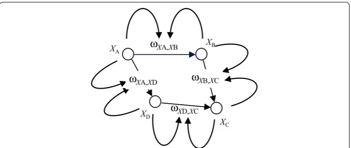
Next an adaptive temporal–causal network model is discussed to model evolving social interactions based on the homophily principle. According to this principle, also indi-cated as ‘birds of a feather flock together’, connections are strengthened if the connected states are similar. For example, when two persons both like the same type of music, mov-ies, drinks, and partmov-ies, they may strengthen their connection. For the current model, the dynamic connection weights ωXA,XB from state XA of person A to state XB of person
slogistic(ωX
1,YX1,. . .,ωXk,YXk)=1/
1+e−σ
ωX1,YX1+···+ωXk,YXk−τ
.
c(V1,. . .,Vk)=alogistic(V1,. . .,Vk)=
1
1+e−σ (V1+...+Vk−τ ) −
1
1+eστ
1+e−στ
alogisticσ,τ(V1,. . .,Vk)
c∗Y(V1, V2, W) = cY(WV1, V2)
B are assumed to change over time based on the principle that the closer the activa-tion levels of the states of the interacting persons, the stronger the mutual connecactiva-tions between the persons will become, and the higher the difference between the activation levels, the weaker they will become. For a conceptual representation, see Fig. 3.
As discussed in “Network-Oriented Modelling by temporal–causal networks” section, ωXA,XB can be represented by state XA,XB and the weights of the connections involving
XA,XB are assumed 1: the weights of the connections from XA and XB to XA,XB, and from XA,XB to XB and to itself. Based on this according to the temporal–causal network approach, the homophily principle may be formalised using the following general format and a combination function cA,B(V1,V2,W) that still has to be determined:
Note that the connection weight XA,XB increases when c� XA,XB
XA(t), XB(t),�XA,XB(t)
> �XA,XB(t), decreases when c�XA,XB
XA(t), XB(t),�XA,XB(t)
< �XA,XB(t) and stays the same when c�
XA,XB
XA(t), XB(t),�XA,XB(t)
=�XA,XB(t).
Examples of such combination functions can be obtained when a threshold value τ�XA,XB is assumed such that the connection weight XA,XB becomes stronger when |XA(t)−XB(t)|< τ�XA,XB (levels of XA and XB close to each other) and weaker when |XA(t)−XB(t)|> τ�XA,XB (levels of XA and XB not so close to each other). The following is an example which is linear in XA(t)andXB(t):
The factor β can be made dependent on �XA,XB(t), to keep values of �XA,XB(t) within
the [0, 1] interval: β =α�XA,XB(t)
1−�XA,XB(t)
, with α an amplification parameter.
This makes the combination function
�XA,XB(t+�t)=�XA,XB(t)+η�XA,XB
c�
XA,XB(XA(t), XB(t), �XA,XB)−�XA,XB
�t
d�X A,XB
dt=η
�XA,XB
c�
XA,XB(XA, XB, �XA,XB)−�XA,XB
c�XA,XB(XA(t),XB(t),�XA,XB(t))=�XA,XB(t) +β(τ�XA,XB− |XA(t)−XB(t)|)
Table 1 Overview of a number of standard combination functions Name Description Formula c(V1,…, Vk)=
sum(..) Sum V1+ · · · +Vk
product(..)
cproduct(..) ProductComplement product V1
∗ · · · ∗Vk
1−(1−V1)∗ · · · ∗(1−Vk)k)
min(..)
max(..) Minimal valueMaximal value min(max(VV11,…, V,…, Vkk))
slogisticσ,τ(..) Simple logistic sum 1 1+e−σ (V1+···+Vk−τ ) with σ, τ≥ 0 alogisticσ,τ(..) Advanced logistic sum 1 1+e−σ (V1+···+Vk−τ )
−
1
(1+eσ τ)
1+e−σ τ
with σ, τ≥ 0
ssumλ(..) Scaled sum (V1+⋯+Vk)/λ with λ > 0
sisum(..) Scaled sum with interac-tion terms (
V1+⋯+Vk)/λ+ ΣijμijViVj with λ > 0
aproductβ(..) Advanced product βcproduct(V1,…, Vk)+(1 −β) product(V1,…, Vk) with
0 ≤β≤1
aminmaxβ(..) Advanced minimum and
maximum βmax(V1,…, Vk)+ (1 −β) min(V1,…, Vk) with 0 ≤ β≤1
aproduct‑ssumβ,λ(..) Advanced product and
scaled sum aproductβ(
where V1,V2 refer to XA,XB and W to XA,XB. Thus, we obtain the following:
The combination function for XB can be found in the same way as in the “ Network-Oriented Modelling by temporal–causal networks” section for Y.
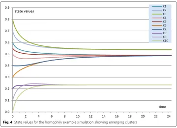
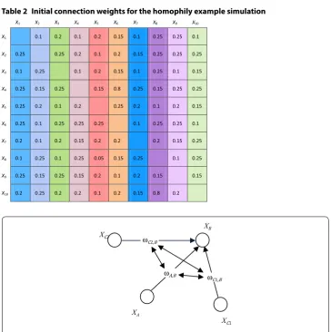
In Figs. 4 and 5, as an illustration, an example simulation for this homophily model is shown, based on a (fully connected) example network of 10 states X1 to X10, with the ini-tial values of the connection weights shown in Table 2. For the contagion between states, a dynamic scaled sum function has been used in which, at each point in time, the scaling factor is equal to the sum of the connection weights involved. The homophily threshold τ was set at 0.025, and the amplification factor α at 20. Speed factors for states were 0.5 and for connections 0.3.
All connection weights approximate either 0 or 1, as can be seen for a few examples (of the 90 connections) in Fig. 5. In Fig. 4, it is shown that clustering emerges, in this case in 3 clusters that in the end each are fully connected by connection weights 1, and the con-nection weights between states from different clusters have become practically 0. That such patterns always occur will be analysed further in the “Mathematical analysis for the homophily principle” section.
Modelling evolving social interactions by adaptive networks based on the ‘more becomes more’ principle
Another type of model for a dynamic connection from a person B to A takes into account to which extent other persons C connect to person A. The idea behind this is that some-body who is very popular seems worth connecting to. Sometimes this is called the ‘more becomes more’ principle, and in a wider context it relates to what sometimes is called ‘the rich get richer’ (Simon [27]), ‘cumulative advantage’ (Price [28]), ‘the Matthew effect’ (Merton [29]) or ‘preferential attachment’ (Barbasi [30]). For example, if B is followed by
c�XA,XB(V1,V2, W)=W+αW(1−W) (τ�XA,XB − |V1−V2|)
�XA,XB(t+�t)=�XA,XB(t)+η�
XA,XB[α�XA,XB(t)(1−�XA,XB(t)) (τ�XA,XB − |XA(t)−XB(t)|)]�t
d�XA,XB/dt =η�
XA,XB[α�XA,XB(t)(1−�XA,XB(t)) (τ�XA,XB− |XA(t)−XB(t)|)].
ω
XA,XBω
XB,XCXA XB
XC
XD
ω
XA,XDω
XD,XCmany others C on Twitter, then B seems to be interesting to follow for A as well. As the connections of others to B may change over time, this will imply that A also will have a dynamic connection to B, and in turn this connection will affect the connection of oth-ers to B over time as well. This can be modelled taking into account the weights ωCi,B for
i = 1,…, k of all connections from others Ci to B as shown in Fig. 6 in conceptual repre-sentation and in numerical reprerepre-sentation as follows:
dωA,B/dt=ηA,B[cA,B(ωC1,B. . .,ωCk,B)−ωA,B]
ωA,B(t+�t)=ωA,B(t)+η
A,B[cA,B(ωC1,B(t),. . .,ωCk,B(t))−ωA,B(t)].
0.0 0.1 0.2 0.3 0.4 0.5 0.6 0.7 0.8 0.9
0 2 4 6 8 10 12 14 16 18 20 22 24
X1 X2 X3 X4 X5 X6 X7 X8 X9 X10
state values
me
Fig. 4 State values for the homophily example simulation showing emerging clusters
0.0 0.1 0.2 0.3 0.4 0.5 0.6 0.7 0.8 0.9 1.0
0 2 4 6 8 10 12 14 16 18 20 22 24 26 28 30 32 34 36 38
X2_X3 X3_X4 X4_X5 X5_X4 X8_X5
connecon weight values
me
Here cA,B(…) is a combination function for the values ωC1,B,. . .,ωCk,B; for exam-ple, a logistic sum function or a scaled sum function with scale factor the number k of other persons connected to B. Note that the latter combination function only takes into account the average strengths of the connections, not the total number of them.
Note that a network modelling the initiation of connections is not automatically a net-work indicating social contagion; this will depend on the application considered. For example, a network modelling a connection from A to B when A is following B on Twit-ter will not play a role in social contagion from A to B. For social contagion, the opposite network plays a role where a connection from A to B occurs when A is followed by B, which is not initiated by A but by B: on Twitter and most other social media you cannot
ssum(V1,. . .,Vk)=(V1+ · · · +Vk)/
alogistic(V1,. . .,Vk)=
1
1+e−σ (V1+···+Vk−τ ) − 1 1+eσ τ
(1+e−σ τ).
Table 2 Initial connection weights for the homophily example simulation X1 X2 X3 X4 X5 X6 X7 X8 X9 X10
X1 0.1 0.2 0.1 0.2 0.15 0.1 0.25 0.25 0.1
X2 0.25 0.25 0.2 0.1 0.2 0.15 0.25 0.25 0.25
X3 0.1 0.25 0.1 0.2 0.15 0.1 0.25 0.1 0.15
X4 0.25 0.15 0.25 0.15 0.8 0.25 0.15 0.25 0.25
X5 0.25 0.2 0.1 0.2 0.25 0.2 0.1 0.2 0.15
X6 0.25 0.1 0.25 0.25 0.25 0.1 0.25 0.25 0.1
X7 0.2 0.1 0.2 0.15 0.2 0.2 0.2 0.15 0.25
X8 0.1 0.25 0.1 0.25 0.05 0.15 0.25 0.1 0.25
X9 0.25 0.15 0.25 0.15 0.2 0.1 0.2 0.15 0.15
X10 0.2 0.25 0.2 0.2 0.1 0.2 0.15 0.8 0.2
XC2
XB
XC1
XA
ωA,B
ωC2,B
ωC1,B
appoint your own followers. As another example, when A often contacts B for advice, and this advice is often taken over by A, then the initiation connection is from A to B but the contagion connection is from B to A. In other cases, it may be different. For example, if
A wants to announce an event or new product, he or she can choose an occasion where many others will see the message; for example, posting it on a suitable forum; in such a case both the initiation and the social contagion are directed from A to the others.
Mathematical analysis of temporal–causal network models
In this section, we discuss how some types of dynamic properties of adaptive temporal– causal network models can be analysed mathematically, in particular, stationary points and monotonicity. These are basic concepts that also can be found in [1], chapter 12 or [31] . A stationary point of a state occurs at some point in time if for this time point no change occurs: the graph is horizontal at that point. Stationary points are usually maxima or min-ima (peaks or dips) but sometimes also other stationary points may occur. An equilibrium occurs when for all states no change occurs. From the difference or differential equations describing the dynamics for a model, it can be analysed when stationary points or equilib-ria occur. Moreover, it can be found when a certain state is increasing or decreasing, when a state is not in a stationary point or equilibrium. First a definition for these notions.
Definition (stationary point, increase, decrease, and equilibrium)
• A state Y has a stationary point at t if dY(t)/dt=0.
• A state Y is increasing at t if dY(t)/dt>0.
• A state Y is decreasing at t if dY(t)/dt<0.
The model is in equilibrium at t if every state Y of the model has a stationary point at
t. This equilibrium is attracting when for any state Y, all values of Y in some neighbour-hood of the equilibrium value increase when the value is below the equilibrium value and decrease when the value is above the equilibrium value.
A question that can be addressed is whether observations based on one or more simu-lation experiments are in agreement with a mathematical analysis. If it is found out that the observations are in agreement with the mathematical analysis, then this provides some extent of corroboration that the implemented model is correct. If they turn out not to be in agreement with the mathematical analysis, then this indicates that prob-ably there is something wrong, and further inspection and correction has to be initiated. Considering the differential equation for a temporal–causal network model, more spe-cific criteria can be found:
where X1,…, Xk are the states with connections to Y. For example, it can be concluded that
In this manner, the following criteria can be found: dY(t)/dt =η
Y[cY(ωX1,YX1(t),. . .,ωX
k,YXk(t)) −Y(t)]
dY(t)/dt>0⇔cY(ωX1,YX1(t),. . .,ωX
Criteria for increase, decrease, stationary point and equilibrium
Let Y be a state and X1,. . .,Xk the states connected toward Y. Then, the following hold:
Note that these criteria can immediately be found from a conceptual representation of a temporal–causal network model, as long as the referred combination function is known. Using the above criteria, no further numerical representation is needed of the difference or differential equations, for example. From these criteria, more insight can be obtained about the behaviour of the network model, in particular which stationary points are possible for a state in the model, and which equilibria are possible for the whole model. Sometimes, the stationary point equation can be rewritten into an equa-tion of the form Y(t) = .. such that Y(t) does not occur on the right-hand side. In the “Mathematical analysis for the homophily principle” and “Mathematical analysis for the ‘more becomes more’ principle” sections, examples of this are shown.
The criteria can also be used to verify (the implementation of) the model based on inspection of stationary points or equilibria, in two different manners A and B. Note that in a given simulation the stationary points that are identified are usually approximately stationary; how closely they are approximated depends on different aspects, for example, on the step size, or on how long the simulation is done.
A. Verification by checking stationary points through substitution of the values from a simulation in the criterion
1. Generate a simulation.
2. Consider any state Y with a stationary point at any time point t and states X1, …,Xk
affecting it.
3. Substitute the values Y(t) and X1(t), …, Xk(t) in the criterion cY(ωX1,YX1(t),. . .,ωXk,YXk(t))=Y(t).
4. If the equation holds (for example, with an accuracy <0.05), then this test succeeds, otherwise it fails
5. If this test fails, then it has to be explored were the error can be found
Note that this method A. works without having to solve the equations, only substitu-tion takes place; therefore it works for any choice of combinasubstitu-tion funcsubstitu-tion. Moreover, note that the method also works when the values of the states fluctuate, for exam-ple according to a recurring pattern (a limit cycle). In such cases for each state, there are maxima (peaks) and minima (dips), which also are stationary points to which the method can be applied; here it is important to choose a small step size as each stationary point occurs at one time point only. There is still another method B. possible that can be applied sometimes; it is based on solving the equations for the stationary point values by symbolic rewriting. This can provide explicit expressions for stationary point values in
Y has a stationary point att⇔cY(ωX1,YX1(t),. . .,ωXk,YXk(t))=Y(t)
Y is increasing att⇔cY(ωX1,YX1(t),. . .,ωXk,YXk(t)) >Y(t)
Y is decreasing att⇔cY(ωX1,YX1(t),. . .,ωXk,YXk(t)) <Y(t)
The model is in equilibrium at⇔cY(ωX1,YX1(t),. . .,ωXk,YXk(t))=Y(t)
terms of the parameters of the model. Such expressions can be used to predict equilib-rium values for specific simulations, based on the choice of parameter values.
B. Verification by solving the equilibrium equations and comparing predicted equilibrium values to equilibrium values in a simulation
1. Consider the equilibrium equations for all states Y:
2. Leave the t out and denote the values as constants
An equilibrium is a solution X1,. . .,Xk of the following set of n equilibrium equations in the n states X1,. . .,Xn of the model:
3. Solve these equations mathematically in an explicit analytical form: for each state Xi
a mathematical formula Xi = … in terms of the parameters of the model (connection
weights and parameters in the combination function cXi(..), such as the steepness σ and threshold τ in a logistic sum combination function); more than one solution is possible.
4. Generate a simulation.
5. Identify equilibrium values in this simulation.
6. If for all states Y, the predicted value Y from a solution of the equilibrium equations equals the value for Y obtained from the simulation (for example, with an accu-racy <0.05), then this test succeeds, otherwise it fails.
7. If this test fails, then it has to be explored where the error can be found.
For more details, see [1], chapter 12, or [31]. This method B. provides more, but a major drawback is that it cannot be applied in all situations; this depends on the chosen combination functions: e.g. for logistic functions, it does not work.
Mathematical analysis for the homophily principle
In the “Modelling evolving social interactions by adaptive networks based on the ‘more becomes more’ principle” section, it was shown how the homophily principle for evolv-ing social interaction may be modelled usevolv-ing a combination function:
In this section, we analyse which stationary points can occur for XA,XB, according to the approach described in “Mathematical analysis of temporal–causal network models”. For this case, the criterion from the “Mathematical analysis of temporal–causal network models” section for a stationary point is
cY(ωX1,YX1(t),. . .,ωXk,YXk(t))=Y(t).
cY(ωX1,YX1,. . .,ωXk,YXk)=Y.
cX
1(ωX1,X1X1,. . .,ωXn,X1Xn)=X1 . . .
cX
n(ωX1,XnX1,. . .,ωXn,XnXn)=Xn
c�XA,XB(V1,V2,W)=W +W(1−W)
τ�XA,XB − |V1−V2|
Clearly, for �XA,XB(t)=0 or �XA,XB(t)=1, one of the left-hand side factors in this con-dition is 0. In contrast, when 0< �XA,XB(t) <1, the right-hand factor should equal 0:
Therefore, in principle, there are three types of stationary points for �XA,XB(t). Stationary points for�XA,XB(t):
Similarly, the following can be found.
Increasing�XA,XB(t)
Decreasing�XA,XB(t)
This shows that for cases that |XA(t)−XB(t)|< τ�XA,XB the connection keeps on becoming stronger until �XA,XB(t) approaches 1. Similarly for cases that |XA(t)−XB(t)|> τ�XA,XB the connection keeps on becoming weaker until �XA,XB(t)
approaches 0. This implies that �XA,XB(t)= 0 and �XA,XB(t)=1 can both become
attracting, but under different circumstances concerning the values of XA(t) and XB(t) . In [1], chapter 11, section 11.7 for such an adaptive network model, an example simula-tion is shown where indeed the connecsimula-tion weights all converge to 0 or 1, and during this process clusters are formed of persons with equal levels of their state; see also [32].
Mathematical analysis for the ‘more becomes more’ principle
The criterion for stationary points applied to the adaptive network model for the ‘more becomes more’ principle is the following:
where C1,. . .,Ck, and A are the states connected to B. For a joint stationary point, this
criterion applies to any state connected to B. Renaming A by Ck+1 this can also be for-mulated by the following set of k+1 equations for i=1,. . .,k+1:
or written out:
c�
XA,XB
XA(t),XB(t),�XA,XB(t)
=�XA,XB(t)
⇔�XA,XB(t)
1−�XA,XB(t)
τ�XA,XB− |XA(t)−XB(t)|
=0
τ�XA,XB − |XA(t)−XB(t)| =0⇔ |XA(t)−XB(t)| =τ�XA,XB.
�XA,XB(t)=0 or�XA,XB(t)=1 or|XA(t)−XB(t)| =τ�XA,XBand�XA,XB(t)have any value.
d�XA,XB(t)/dt>0⇔(τ�XA,XB − |XA(t)−XB(t)|) >0⇔ |XA(t)−XB(t)|< τ�XA,XB
d�XA,XB(t)/dt<0 ⇔
τ�XA,XB− |XA(t)−XB(t)|
<0⇔ |XA(t)−XB(t)|> τ�XA,XB
cA,BωC1,B(t),. . .,ωCk,B(t)
=ωA,B(t)
cCi,BωC1,B(t),. . .,ωCi−1,B(t),ωCi+1,B(t),. . .,ωCk+1,B(t)
=ωCi,B(t)
cC1,B(ωC2,B(t),. . .,ωCk+1,B(t))=ωC1,B(t)
cC2,B(ωC1,B(t),ωC3,B(t),. . .,ωCk+1,B(t))=ωC2,B(t)
. . .
If for the combination function cCi,B(..) the scaled sum function is chosen with scaling factor the number k, this provides the following set of k + 1 linear equations for a joint stationary state for the connections to B:
By multiplying both sides by k this provides
This set of equations can be solved easily. For each i, adding ωCi,B(t) to both sides of the ith equation yields
As all left-hand sides are equal now, it follows that the right-hand sides are equal as well, so for a joint stationary point
for all i and j. Therefore in a joint stationary state for all connections ωCi,B to B they have the same weight value.
By a slightly different argument a similar conclusion can be drawn when not a scaled sum combination function but a logistic combination function is chosen.
The aggregated impact on the connection weight ωCi,B is given by (ωC2,B(t)+ · · · +ωCk+1,B(t))/k=ωC1,B(t)
(ωC1,B(t)+ωC3,B(t)+ · · · +ωCk+1,B(t))/k=ωC2,B(t)
. . .
(ωC1,B(t)+ · · · +ωCk,B(t))/k=ωCk+1,B(t)
(ωC2,B(t)+ · · · +ωCk+1,B(t))=kωC1,B(t)
(ωC1,B(t)+ωC3,B(t)+ · · · +ωCk+1,B(t))=kωC2,B(t)
. . .
(ωC1,B(t)+ · · · +ωCk,B(t))=kωCk+1,Bt
ωC1,B(t)+ωC2,B(t)+ · · · +ωCk+1,B(t)=kωC1,B(t)+ωC1,B(t))=(k+1)ωC1,B(t) ωC1,B(t)+ωC2,B(t)+ · · · +ωCk+1,B(t)=kωC2,B(t)+ωC2,B(t)=(k+1)ωC2,B(t)
. . .
ωC1,B(t)+ωC2,B(t)+ · · · +ωCk+1,B(t)=kωCk+1,B(t)+ωCk+1,B(t)= (k+1)ωCk+1,B(t).
ωCi,B(t)=ωCj,B(t)
alogistic
ωC1,B(t),. . .,ωCi−1,B(t),ωCi+1,B(t),. . .,ωCk,B(t)
=
1 1+e−σ
ωC1 ,B+···+ωCi−1 ,B+ωCi+1 ,B+···+ωCk,B−τ
−
1
(1+eσ τ)
1+e−σ τ
=
1 1+e−σ
ωC1 ,B+···+ωCi−1 ,B+ωCi,B+ωCi+1 ,B+···+ωCk,B−τ−ωCi,B
−
1
(1+eσ τ)
×1+e−σ τ
=
1 1+e−σ
�−ωCi,B
−µ
v
=
1 1+e−σ �eσωCi,B −µv
=
1 1+κeσωCi,B
−µ
v
with f(V) a function defined by
Here κ, μ, ν are positive constants:
Using this function, for this case, the stationary point equations get the following uni-form uni-form:
Therefore, the question becomes how many solutions the equation f(V) =V has. Now eσV is monotonically increasing in V, and therefore 1/(1+κeσV)) and also f(V) are monotonically decreasing: V1≤V2⇒f(V1)≥f(V2). Suppose V1 and
V2 are two solutions of the equation f(V)=V, and assuming V1≤V2, it follows V1=f(V1)≥f(V2)=V2, soV1=V2. This implies that the equation f(V)=V has at most one solution. From this, it follows that also for the alogistic function as combina-tion funccombina-tion in a joint stacombina-tionary point all ωCi,B values will be equal.
There is also an abstract general argument possible for a whole class of combination functions, namely, the combination functions that are (1) symmetric in their arguments and that are (2) monotonic:
1. If U1,. . .,Uk is a permutation of V1,. . .,Vk, then c(U1,. . .,Uk)=c(V1,. . .,Vk)
2. If it holds Ui≤Vi for all i, then c(U1,. . .,Uk)≤c(V1,. . .,Vk)
If in a fully connected network a combination function c(..) is used that is symmetric and monotonic and all connection weights between different states are the same (for example, assume all of them 1), and no connections occur from states to themselves, then the argument is as follows. Suppose all states have the same combination function and joint stationary points are given, so that for all i and j (assume i < j):
then by symmetry
Now suppose Xi≤Xj then by monotonicity
f(V)=
1
1+κeσV −µ
ν
κ=e−σ �with�=ωC1,B+ · · · +ωCk,B−τ
µ=1/(1+eσ τ)
ν=(1+e−σ τ).
f(ωC1,B(t))=ωC1,B(t)
. . . . . . . . .
f(ωCk,B(t))=ωCk,B(t).
Xi=c(X1,. . .,Xi−1,Xi+1,. . . .,Xk)
Xj=c(X1,. . . .,Xj−1,Xj+1,. . .,Xk)
From the above, it follows that Xi=Xj. The same argument applies when it is assumed
Xi≥Xj. Therefore in this case, in a joint stationary point all state values are equal, which
was also found above by more specific methods for the special cases of a scaled sum and an advanced logistic sum combination function, which indeed both are symmetric and monotonic combination functions. Thus, we obtain the following theorem:
Theorem When in a fully connected network with equal connection weights a combina-tion funccombina-tion is used that is symmetric and monotonic, then in a joint stacombina-tionary point all state values are equal.
‘More becomes more’ and scale‑free networks
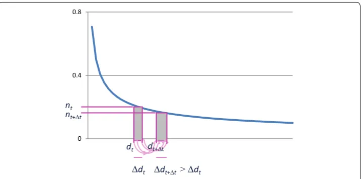
The ‘more becomes more’ principle has also been used to provide an explanation for the empirical evidence that most real-world networks are scale-free. The idea is that the typ-ical distribution of degrees according to a power law emerges from an evolving network when it is assumed that the network dynamics is based on some form of a ‘more become more’ principle (also called preferential attachment); see, for example, [30, 33–35]; see also [36, 37]. An indication of the type of argument followed is illustrated in Fig. 7. Here the distribution of nodes (vertical axis) over degrees (horizontal axis) is depicted; this distribution is assumed stable over time. A time point t is considered and the focus is at the nodes with some degree dt at t (see at the horizontal axis). There is a (relative) num-ber or density nt of them (vertical axis). Moreover, the nodes with degree between dt and a bit higher dt+dt are considered, an interval of length dt at the horizontal axis. The (relative) number of nodes with degree within this interval is represented in Fig. 7 by the area of the (left) rectangle above that interval. This area is approximated by ntdt.
Now consider a time step from t to t+t. Due to growth of the number of connec-tions, the nodes with degree dt at time t will have a higher degree dt+t at t+t, and the nodes with degree dt+dt at time t will have a higher degree dt+t+dt+t at
t+t. Due to the ‘more becomes more’ principle, from dt <dt+�dt it follows that from t to t + ∆t the nodes with degree dt+dt at time t will get more new connections than the nodes with degree dt at time t. Therefore the increase in degree of these nodes with degree dt+dt at time t will be higher:
The numbers of nodes previously represented at t by the left rectangle are represented at t+t by the right rectangle. Moreover, because they describe the same nodes, the areas indicated as shaded are the same:
Given this equality, from �dt+�t> �dt (‘more becomes more’ principle) it follows that nt+�t<nt. Therefore the distribution is monotonically decreasing. By a more
Xi=c(X1,. . .,Xi−1,Xi+1,. . .,Xj−1,Xj+1,. . .,Xk,Xj) ≥c(X1,. . .,Xi−1,Xi+1,. . .,Xj−1,Xj+1,. . .,Xk,Xi)
=Xj
�dt+�t> �dt
complex argument it has been derived that based on some more precise assumptions on the formalisation of the ‘more becomes more’ principle, a distribution is obtained that is monotonically decreasing according to a power law; for example, see [30, 33–35] for more details.
Discussion
The Network-Oriented Modelling approach based on adaptive temporal–causal net-works, as described here (see also [1, 10]), provides a dynamic modelling approach that enables a modeller to design high-level conceptual model representations in the form of cyclic graphs (or connection matrices). These conceptual representations can be system-atically transformed in an automated manner into executable numerical representations that can be used to perform simulation experiments. The modelling approach makes it easy to take into account. on the one hand. theories and findings from any domain from, for example, biological, psychological, neurological or social sciences, as such theories and findings are often formulated in terms of causal relations. This applies, among oth-ers, to mental processes based on complex brain networks, which, for example, often involve dynamics based on interrelating and adaptive cycles, but equally well it applies to the adaptive dynamics of social interactions. For a more detailed theoretical analysis on the wide applicability of the approach, see [38, 39]; for example, there it is shown that any smooth (state-determined) dynamical system can be modelled by a temporal–causal network model.
This enables to address complex adaptive phenomena within all kinds of integrated cognitive, affective and social processes. By using temporal–causal relations from those domains as a main vehicle and structure for network models, the obtained network models get a strong relation to the large body of empirically founded knowledge from the Neurosciences and Social Sciences. This makes them scientifically justifiable to an extent that is not attainable for black box models which lack such a relation.
In this paper, we have discussed in some detail how mathematical analysis can be used to find out some properties of the dynamics of a network model designed according to a Network-Oriented Modelling approach based on temporal–causal networks; see also
0 0.4 0.8
dt
∆dt ∆dt+∆t > ∆dt nt
nt+∆t
dt+∆t
[1], chapter 12, or [31]. An advantage is that such an analysis is done without performing simulations. This advantage makes that it can be used as an additional source of knowl-edge, independent of a specific implementation of the model. By comparing properties found by mathematical analysis and properties observed in simulation experiments a form of verification can be done. If a discrepancy is found, for example, in the sense that the mathematical analysis predicts a certain property but some simulation does not sat-isfy this property, this can be a reason to inspect the implementation of the model care-fully (and/or check whether the mathematical analysis is correct). Having such an option can be fruitful during a development process of a model, as to acquire empirical data for validation of a model may be more difficult or may take a longer time.
Adaptive network models combining the homophily and the ‘more becomes more’ principle also have been studied recently, in particular in [40, 41]. The methods described in the current paper can and actually have also be applied to such integrated cases. Moreover, it has been shown in [40, 41] how the modelling approach can be related to empirical real-world data on evolving friendship networks.
Mental processes can also be modelled by temporal–causal networks in an adaptive manner. The parameters that can change can be modelled in the same way as states, fol-lowing the approach in “Network-Oriented Modelling by temporal–causal networks” section. This can be applied, for example to the way in which connection strengths can change based on Hebbian learning. Hebbian learning [42], is based on the principle that strengthening of a connection between neurons over time may take place when both states are often active simultaneously (‘neurons that fire together, wire together’). The principle itself goes back to Hebb [42], but see also, e.g. [43]. For some more details on this, see [31].
Acknowledgements None.
Competing interests
The author declares no competing interests.
Publisher’s Note
Springer Nature remains neutral with regard to jurisdictional claims in published maps and institutional affiliations.
Received: 16 February 2017 Accepted: 31 May 2017
References
1. Treur J. Network-oriented modelling: addressing complexity of cognitive, affective and social interactions. Under-standing complex systems series. Berlin: Springer; 2016.
2. Treur J. Network-oriented modelling and its conceptual foundations. In: Proceedings of the 8th international confer-ence on social informatics, SocInfo’16. Lecture Notes in AI. Springer Publishers; 2016.
3. Chung B, Choi H, Kim S. Workflow-enabled internet service delivery for a variety of access networks. In: Proceeding APNOMS’03; 2003.
4. Elzas MS. Organizational structures for facilitating process innovation. Real time control of large scale systems. Heidelberg: Springer; 1985. p. 151–63.
6. Cottret L, Jourdan F. Graph methods for the investigation of metabolic networks in parasitology. Parasitology. 2010;137(09):1393–407.
7. Felsen LB, Mongiardo M, Russer P. Electromagnetic field representations and computations in complex structures I: complexity architecture and generalized network formulation. Int J Numer Model Electron Netw Devices Fields. 2002;15(1):93–107.
8. Felsen LB, Mongiardo M, Russer P. Electromagnetic field computation by network methods. Berlin: Springer Science and Business Media; 2009.
9. Russer P, Cangellaris AC. Network oriented modeling, complexity reduction and system identification techniques for electromagnetic systems. In: Proceedings 4th international workshop on computational electromagnetics in the time-domain; 2001. p. 105–22.
10. Treur J. Dynamic modelling based on a temporal–causal network modelling approach. Biol Inspi Cognit Archit. 2016;16:131–68.
11. Brauer F, Nohel JA. Qualitative theory of ordinary differential equations. Berlin: Benjamin; 1969. 12. Lotka AJ. Elements of physical biology. Dover: Williams and Wilkins (1924); 1956.
13. Picard E. Traité d’Analyse. 1891;1. 14. Picard E. Traité d’Analyse. 1893;2.
15. Poincaré H. Mémoire sur les courbes défine par une équation différentielle. 1881–1882. 16. Poincaré H. New Methods of Celestial Mechanics, 3 vols (English translation). 1967.
17. Treur J. Network-oriented modeling and analysis of dynamics based on adaptive temporal–causal networks. In: Complex Networks & their Applications V. Proceedings of the 5th international workshop on complex networks and their applications. Studies in Computational Intelligence, vol. 693. Berlin: Springer Publishers; 2016. p. 69–82. 18. Beer RD. On the dynamics of small continuous-time recurrent neural networks. Adapt Behav. 1995;3:469–509. 19. Dubois D, Lang J, Prade H. Fuzzy sets in approximate reasoning, part 2: logical approaches. Fuzzy Sets Syst.
1991;40:203–44.
20. Dubois D, Prade H. Possibility theory, probability theory and multiple-valued logics: a clarification. Ann Math Artif Intell. 2002;32:35–66.
21. Giangiacomo G. Fuzzy logic: mathematical tools for approximate reasoning. Dordrecht: Kluwer Academic Publish-ers; 2001.
22. Grossberg S. On learning and energy-entropy dependence in recurrent and nonrecurrent signed networks. J Stat Phys. 1969;1:319–50.
23. Hirsch M. Convergent activation dynamics in continuous-time networks. Neural Netw. 1989;2:331–49. 24. Hopfield JJ. Neural networks and physical systems with emergent collective computational properties. Proc Nat
Acad Sci (USA). 1982;79:2554–8.
25. Hopfield JJ. Neurons with graded response have collective computational properties like those of two-state neu-rons. Proc Nat Acad Sci (USA). 1984;81:3088–92.
26. Zadeh L. Fuzzy sets as the basis for a theory of possibility. Fuzzy Sets Syst. 1978;1:3–28 (Reprinted in Fuzzy Sets Syst 1999;100(Supplement): 9–34).
27. Simon HA. On a class of skew distribution functions. Biometrika. 1955;42:425–40.
28. de Price DJ. A general theory of bibliometric and other cumulative advantage processes. J Am Soc Inform Sci. 1976;27:292–306.
29. Merton RK. The Matthew effect in science. Science. 1968;159:56–63.
30. Barabási AL, Albert R. Emergence of scaling in random networks. Science. 1999;286:509–12.
31. Treur J. Verification of temporal–causal network models by mathematical analysis. Vietnam J Comput Sci. 2016;3:207–21. doi:10.1007/s40595-016-0067-z.
32. Sharpanskykh A, Treur J. Modelling and analysis of social contagion in dynamic networks. Neurocomput J. 2014;146:140–50.
33. Krapivsky PL, Redner S, Leyvraz F. Connectivity of growing random networks. Phys Rev Lett. 2000;85(21):4629–32. 34. Krapivsky PL, Redner S. Organization of growing random networks. Phys Rev E. 2001;63(6):066123.
35. Krapivsky PL, Redner S. Rate equation approach for growing networks. In: Pastor-Satorras R, Rubi M, Diaz-Guilera A, editors. Statistical mechanics of complex networks. Lecture Notes in Physics, vol. 625; 2003. p. 3–22.
36. Bornholdt S, Ebel H. World Wide Web scaling exponent from Simon’s 1955 model. Phys Rev E. 2001;64(3):035104. 37. Newman MEJ. The structure and function of complex networks. Siam Rev. 2003;45(2):167–256.
38. Treur J. Do network models just model networks? On the applicability of network-oriented modeling. In: Proceed-ings of the international conference on network science, NetSci-X-2017. Lecture Notes in Computer Science. Springer Publishers; 2017.
39. Treur J. On the applicability of network-oriented modeling based on temporal–causal networks: why network models do not just model networks. J Inform Telecommun. 2017;1:23–40.
40. Blankendaal R, Parinussa S, Treur J. A temporal–causal modelling approach to integrated contagion and network change in social networks. In: Proceedings of the 22nd European conference on artificial intelligence, ECAI 2016. Frontiers in artificial intelligence and applications, vol. 285. IOS Press; 2016. p. 1388–96.
41. van den Beukel S, Goos S, Treur J. Understanding homophily and more-becomes-more through adaptive temporal– causal network models. In: Proceedings of the 15th international conference on practical applications of agents and multi-agent systems, PAAMS’17. Lecture Notes in Computer Science. Springer Publishers; 2017.
42. Hebb D. The Organisation of Behavior. Hoboken: Wiley; 1949.