A SOLUTION TO THE PROBLEM OF INTERPRETING
VERY LONG TIME SERIES OF AMBIENT NOISE
AS MEASURED AT VERY SPARSE NETWORKS
by
Kathryn Teresa Decker
A dissertation
submitted in partial fulfillment of the requirements for the degree of Doctor of Philosophy in Geophysics
Boise State University
Kathryn Teresa Decker
BOISE STATE UNIVERSITY GRADUATE COLLEGE
DEFENSE COMMITTEE AND FINAL READING APPROVALS
of the dissertation submitted by
Kathryn Teresa Decker
Dissertation Title: A Solution to the Problem of Interpreting Very Long Time Series of Ambient Noise As Measured At Very Sparse Networks
Date of Final Oral Examination: 01 February 2013
The following individuals read and discussed the dissertation submitted by student Kathryn Teresa Decker, and they evaluated her presentation and response to questions during the final oral examination. They found that the student passed the final oral examination.
Paul Michaels, Ph.D. Chair, Supervisory Committee John Bradford, Ph.D. Member, Supervisory Committee
Leming Qu, Ph.D. Member, Supervisory Committee
Michael West, Ph.D. External Examiner
I am happy to acknowledge several individuals and organizations that contributed
im-mensely to my success as a graduate student at Boise State University. Without the help of
the community here at BSU and the funding provided by both internal and external sources,
I never would have accomplished my goals.
I would like to thank my committee members, Dr. John Bradford and Dr. Leming Qu,
who have been enthusiastic and reliable throughout my time at Boise State University. I am
especially grateful for my former and current committee chairs: Dr. Matt Haney, currently
with the USGS, and Dr. Paul Michaels. Dr. Haney was responsible for securing funding
from ION Geophysical and the ARRA Grant for my research, and his enthusiasm for new
projects has introduced me to the world of seismology. Dr. Michaels has been a remarkable
source of reassurance and inspiration and I would like to thank him for countless hours and
words of advice on programming, writing, and completing my degree. I would also like to
express my appreciation for his enthusiasm for taking over the duties of committee chair in
the middle of a project and his ability to direct my research in a way that has allowed for a
timely completion of a work of which I can truly be proud.
I would also like to thank the institutions who provided my funding for the duration of
my time at Boise State University: the Inland Northwest Research Alliance, for providing
full scholarship for my first year, the Department of the Interior and US Geological Survey
Boise State University Department of Geosciences for funding my final year. I also would
like to thank Sky Research, for offering me an internship during the summer of 2010.
I have enjoyed all of the opportunities available to me through the Geosciences
depart-ment, and especially through the Center for Geophysical Investigation of the Shallow
Sub-surface (CGISS) during my years here. I owe a great deal of my success to the continued
support of the department, their flexibility with funding my research, and their commitment
to seeing me complete the program. It has been a pleasure to work with all of the students
and faculty and I am excited to see what comes next for each of my colleagues.
Ambient seismic noise techniques are an excellent choice for imaging the subsurface in
ar-eas that are seismically quiet or otherwise unsuitable for active source experiments due to
geographic isolation or environmental sensitivity. Recently, decades-long time series were
made available for download from the Incorporated Research Institutions for Seismology
(IRIS) from permanent network installations, allowing access to long, uninterrupted
record-ings from seismometers around the world. This has spurred the development of an entire
field of applications for passive seismic noise analysis. Over the continental United States,
the USArray project has advanced to provide station coverage in relatively dense and
reg-ularly spaced arrays, but along the Aleutian Island arc in Alaska and other geographically
isolated but seismically active locations, the hazards associated with volcanic eruptions and
the difficulty of accessing stations for repair or replacement throughout most of the year
has allowed only for sparse coverage.
The analysis of ambient seismic recordings generally suits one of two purposes. The
first involves the parameterization of the source of each component of the ambient seismic
noise spectrum and focuses on both the spatial locations and mechanisms of generation.
The second purpose of looking at ambient seismic noise is to create velocity models of
the subsurface below the array. The assumptions required for the traditional approach to
analysis of ambient seismic noise, namely beamforming and the spatial autocorrelation
are not met when only limited permanent network coverage is available. Furthermore, most
studies focused on mapping the subsurface generally assume that the source of ambient
noise is diffuse and azimuthally homogeneous. Here, principal component analysis (PCA)
is used to show that the source of ambient noise is often highly directive. Methods of
incorporating the direction of approach are introduced to allow one to correct the apparent
velocity calculated by the consideration of an omnidirectional source when the energy is
instead strongly directive. To ensure that the energy measured at a remote network is indeed
pervasive energy that travels through the ground rather than local noise, a quality control
algorithm based on the results of PCA is also introduced. The benefits of improving the
reliability of velocity measurements for the subsurface and reducing the size of the dataset
by the introduction of the quality control parameter will greatly enhance the accuracy and
ease with which scientists may determine subsurface velocity profiles at especially sparse
networks with particularly long recording times.
ACKNOWLEDGMENT . . . iv
ABSTRACT . . . vi
LIST OF FIGURES . . . xiii
LIST OF TABLES . . . xx
1 INTRODUCTION . . . 1
1.1 Data Accessibility and New Challenges . . . 1
1.2 Passive Seismic Methods . . . 4
1.3 Motivation . . . 6
1.4 The Island of Akutan . . . 8
1.5 Organization of Dissertation . . . 9
2 SOURCE PARAMETERS AND ARRAY GEOMETRY . . . 11
2.1 Introduction . . . 11
2.2 Sources of Noise . . . 13
2.2.1 Infragravity: 0.005-0.02 Hz . . . 13
2.2.2 Microseisms: 0.04-1.0 Hz . . . 15
2.4 Survey Geometry . . . 21
2.4.1 Selection of Recordings and Data Extraction . . . 23
3 AMBIENT SEISMIC NOISE METHODS: AN HISTORICAL PERSPECTIVE OF STATISTICAL TECHNIQUES . . . 27
3.1 On the Origin of the Term “Ambient Seismic Noise,” Consideration of Its Source, and Its Applications . . . 27
3.2 Spatial Autocorrelation Coefficient Method . . . 30
3.3 Frequency-Wavenumber Spectral Method and Beamforming . . . 32
3.3.1 Beamforming Method . . . 34
3.4 A General Overview of Traditional Processing Steps for the Passive Seis-mic Method . . . 38
3.4.1 Data Preparation for a Single Station . . . 39
3.4.2 Temporal Stacking of Cross Correlations to Obtain the Green’s Function for Station Pairs . . . 40
3.4.3 Frequency-Time Analysis (FTAN) . . . 42
3.4.4 Error Analysis and Quality Control . . . 45
4 METHODOLOGY AND APPLICATION . . . 49
4.1 Introduction . . . 49
4.2 Methodology . . . 51
4.2.1 Principal Component Analysis . . . 51
4.2.2 Quality Control . . . 54
4.3 Application . . . 57
4.3.2 Calculating Phase Velocity Curves . . . 59
4.4 The Importance of Directive Energy for Sparse Networks . . . 66
5 RESULTS . . . 68
5.1 PCA . . . 70
5.2 Quality-Controlled Cross Correlations . . . 74
5.3 Construction of Phase Curves . . . 75
6 DISCUSSION . . . 80
6.1 Introduction . . . 80
6.2 Frequency-Dependent Source Direction . . . 81
6.3 Quality Control . . . 82
6.4 Memory Management . . . 83
6.5 Areas for Future Research . . . 84
6.5.1 Improving Quality Control . . . 84
6.5.2 Applications . . . 86
7 CONCLUSIONS . . . 88
REFERENCES . . . 91
APPENDICES . . . 101
A DATA ACCESS . . . 101
A.0.3 The IRIS Interface . . . 101
A.0.4 Extracting Data from SEED Format . . . 105
B.1 C Codes . . . 107
B.1.1 readsac2.c . . . 107
B.1.2 sub4.h . . . 121
B.1.3 c bsegy.h . . . 127
B.1.4 bsac.h . . . 136
B.2 Matlab Codes . . . 146
B.2.1 delr.m . . . 155
B.2.2 bpfilt3.m . . . 156
B.2.3 pca2staGen.m . . . 158
B.2.4 ratioanalysis.m . . . 160
B.2.5 particlemotion.m . . . 165
B.2.6 plotxcorr gwin12 2.m . . . 167
B.2.7 stationgeom3.m . . . 173
B.2.8 method2.m . . . 182
C GEOLOGY OF THE ALEUTIANS AND ALASKA . . . 184
C.1 Introduction . . . 184
C.2 General Geological Setting . . . 184
C.3 Geology of Aleutian Islands - An Overview . . . 187
C.3.1 Aleutian Ridge . . . 188
C.3.2 Alaska Peninsula-Kodiak Island . . . 194
C.3.3 Geology of Akutan Volcano . . . 196
C.4 Quaternary Volcanism . . . 198
C.5 Eruptive History at Akutan . . . 200
D DERIVATIONS . . . 207
D.1 Introduction . . . 207
D.2 Derivation of the Spatial Autocorrelation Coefficient . . . 207
D.3 Derivation of the Maximum Likelihood Method . . . 209
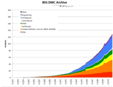
1.1 The IRIS database has expanded exponentially over time as assorted projects
involving long- and short-term installations of seismometers are completed
or underway. . . 3
2.1 The full spectrum for a twenty-minute long signal recorded at station AKUT
on an Streckeisen STS-2 broadband seismometer with sampling interval of
0.02 s. Note that the majority of the signal amplitude occurs for
frequen-cies below 2 Hz. This recording was obtained during a seismically quiet
time period and therefore includes energy from only the ambient seismic
noise sources. . . 17
2.2 The frequencies from DC to approximately 0.02 Hz are pictured here.
Spectral amplitude is found even as one moves towards zero. The very low
frequency components of the amplitude spectrum arise from the excitation
of lower frequency normal modes by ambient seismic sources. . . 18
2.3 A spectral peak is evident at approximately 0.036 Hz (period of
approx-imately 27.8 s) in the spectral amplitude. This is in keeping with what
one would expect for a recording during the northern hemisphere summer
as signal amplitude for the 26 s microseism is highest during the winter
months in the southern hemisphere. . . 18
spectrum for the recording at AKUT at approximately 0.06 Hz and 0.12
Hz, respectively. The SF amplitude is less than that of the DF. The lack of
a particularly evident individual peak for the two features is in agreement
with the relatively broad power spectral density peaks published elsewhere
(see, for example Leeet al., 2011). . . 19
2.5 Plot of the Earth’s hum, the 26 s microseism, and the SF and DF for a
20-minute long time series recorded at station AKUT. Note the relative
amplitude of each of the signals. . . 20
2.6 Stations AKGG, AKLV, AKRB, and AKUT were positioned using the GPS
coordinates of each station as recorded in the header of the data files from
IRIS. . . 22
2.7 IRIS database station coverage for the year of 2009 for the AV network.
The percentages in parentheses on the vertical axis indicate the amount of
coverage during the time of inquiry, in this case ranging from January 1
of 2009 to March 10, 2010. The number of substantial gaps in the records
are also listed on the vertical axis. Although the time series request
even-tually used for this project did not cover this particular time window, it is
worth noting that stations AKGG, AKLV, and AKRB all have continuous
coverage here, as well. This suggests the analysis presented here could be
adapted for investigations of data sets recorded over several years. . . 25
(a) the AV network, and (b) the AT network, over the period of May 16,
2008 - January 16, 2009. Although some gaps exist in the records from the
AV network, all stations had 100% coverage during the period of August
2008 - January 2009. . . 26
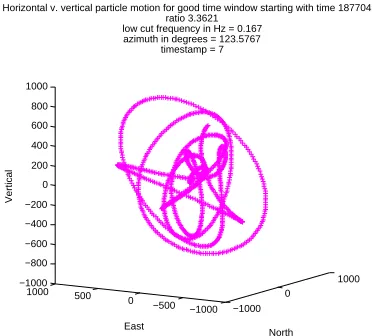
4.1 Plot of particle motion for a window with (a) high maximum-to-minimum
eigenvalue ratio and (b) low maximum-to-minimum eigenvalue ratio for
data filtered over a pass band of 0.167-0.334 Hz. Note that the motion in
(a) is distinctly elliptical and the minor axis of the ellipse is significantly
smaller than the major axis. In (b), the particle motion is more circular than
elliptical because the ratio between the maximum and minimum eigenvalue
is closer to 1. . . 55
4.2 Particle motion for unfiltered good window is much less smooth than the
motion plotted for filtered windows. . . 56
4.3 Example of elliptical particle motion for a portion of recordings on the
vertical, north, and east channels of station AKLV over a good window of
time. Signal has been filtered over a pass band of 0.167-0.334 Hz. . . 58
4.4 Plot of cross correlation between station AKLV and AKUT for the
20-minute period beginning at 6:00 pm on August 4, 2008. Note that the
peak occurs near zero, indicating a very brief delay time between the two
stations. This is in agreement with the directional arrival determined in the
PCA analysis, which indicates an almost broadside arrival of energy for the
station pair AKLV-AKUT. . . 60
played in Figure 4.4. At frequencies higher than approximately 1 Hz, the
amplitude quickly drops off and then remains close to zero. . . 61
4.6 Plot of the unwrapped phase spectrum for the FFT of the cross correlation
displayed in Figure 4.4. This figure shows the unwrapped phase result
for the portion of the frequency bandwidth with the highest amplitude, as
indicated in the plot in Figure 4.5. . . 62
4.7 Schematic of a wave front passing through two stations of arbitrary
orien-tation. Note that the difference in time between the time 1 and time 2 noted
in the figure is the δt of Equation 4.8, and this represents the time lapse
for the same wavefront to pass from one station to another. The distance
labeled ∆A is the distance that a wavefront must travel from Station 1 to
Station 2, and is dependent on the direction, measured as φ degrees from
North, of incoming energy. . . 65
5.1 Plot of earthquakes of all magnitudes recorded from August 1, 2008 to
Au-gust 5, 2008 near the Aleutian Islands, Alaska. Note that no earthquakes
occurred in or around the period from 6:00 - 6:20 am, the time of
measure-ment for the signals used here for analysis. . . 69
5.2 Example of the power spectrum for one channel of one station used in
anal-ysis. Frequency content of all time series was about the same. The majority
of the spectral amplitude occurs within the microseismic bandwidth, as
ex-pected, and spectral amplitude above 2 Hz is almost zero. . . 70
bad time windows for stations AKLV and AKUT. Note that the analysis
to produce these figures was conducted for data that had been filtered with
a fourth order Butterworth bandpass filter with a passband of 0.1-0.2 Hz.
This bandwidth covers portion of the spectra for each station where the
largest spectral amplitudes are found. One may observe that performing
PCA and adding a quality control has selected very few good azimuths.
The bad windows show energy arriving from many sources. Compared to
the plots in Figure 5.4, it is clear that the isolation of a few good azimuths
no longer occurs as one moves to frequencies above the point where the
spectral amplitude begins to decay. This could be a suggestion of the signal
source being mainly local noise above the microseism bandwidth. . . 72
5.4 Histogram rose plots of azimuths at good and bad time windows for
sta-tions AKLV and AKUT. The fourth order Butterworth bandpass filter used
to produce these figures had a passband of 0.75-1.5 Hz, above what is
com-monly accepted as the bandwidth for microseisms. The cutoff point for the
largest spectral amplitudes is around 1 Hz so this bandwidth overlaps into
the area with less signal strength. This shows that the higher frequency
noise is less likely to come from a dominant direction and may indicate
that higher frequency noise is a local effect. . . 73
5.5 Cross correlation for AKRB (southern station) and AKLV (northern
sta-tion). The positive (acausal) lag indicates the energy passes from AKLV to
AKRB rather than from AKRB to AKLV. . . 75
5.6 Cross correlation for the two northernmost stations, AKGG and AKLV. . . 76
in the time series from station AKUT and AKLV. The filter used for the
PCA analysis had a center frequency of 0.7576 Hz and produced several
good windows. Note that there is strong dispersion. At frequencies
be-low about 0.2 Hz, there is little signal, which explains the steep dropoff to
unreasonable slow velocities. . . 77
5.8 Forward model produced for the case of a layer over a half-space. Top layer
shear velocity was set to 500 m/s (appropriate for unsaturated to saturated
sandy material) with a thickness of 600 m. The half-space velocity was set
to 4000 m/s to represent bedrock. . . 78
5.9 Phase velocity dispersion curve from shared good window for station pair
AKRB-AKLV on Julian Day 188 (July 6), 2008 from 12:00 am to 12:20
am. Note possible arrival of a second mode above 0.6 Hz. . . 79
6.1 Phase velocity curve produced from measure ofφ in filtered signals with
center frequency at 0.7576 Hz in one of the windows where each station
reports an eigenvalue ratio that is greater than the cutoff value. Note that
the velocity units are in m/s, so the magnitudes at higher frequencies reach
values that are unrealistic for earth materials, and at lower frequencies there
does not appear to be dispersion, although the dispersion trend is evident
in the frequency range from approximately 0.4-0.6 Hz. This suggests the
need for a multistage selection criteria that incorporates both the original
comparison between a window’s maximum-to-minimum eigenvalue ratio
and the maximum of that ratio at any window as well as a comparison
between the azimuths reported by PCA at each station. . . 84
area of interest. Click the map icon to select a bounding box, which will
automatically enter the latitudes and longitudes of its location, or manually
enter values for latitude and longitude of a bounding box in the region
highlighted by the yellow square. . . 102
A.2 A search for stations on Akutan was conducted over the bounding box
se-lected using the map interface outlined in red. . . 103
C.1 Google Earth image with superimposed stratigraphic columns showing
dif-ferences in geology along Aleutian Arc from east to west. Akutan Island is
indicated. Adapted from Vallier et al., 1998. . . 189
C.2 Spread of ash at (a) 0:00 UTC, (b) 3:00 UTC, (c) 6:00 UTC, (d) 9:00 UTC,
and (e) 12:00 UTC. Plots generated with the Puff Model to represent
pos-sible results of a large Strombolian eruption on Akutan. . . 205
5.1 Example of good and bad window statistics for two stations, AKLV and
AKGG, over different bandwidths. . . 71
C.1 Names and descriptions for formations found in the Aleutian Arc. . . 190
Chapter 1
INTRODUCTION
1.1
Data Accessibility and New Challenges
Over the past 40 years, the field of seismology has changed dramatically due to the
intro-duction of digital recording technologies and incredible increases in the memory storage
capabilities of personal computers. The science is now on the verge of a second
revolu-tion: data storage is no longer limited by the finite memory of one’s personal computer
or external storage device, but instead can be stored in the computing cloud and accessed
almost instantly through the internet. The primary publically accessible source of seismic
data is a massive online database of recordings from seismometers installed at permanent
or semipermanent arrays around the world, organized and maintained by the Incorporated
Research Institutions for Seismology (IRIS). In addition to the historic data holdings, IRIS
also collects data in real-time from stations in networks established in particularly
seismi-cally active regions.
The International Association for Seismology and Physics of the Earth’s Interior’s
(IASPEI) adoption of an internationally recognized format for digital seismic data in 1987
Institu-tions for Seismology, 2010). The continually increasing volume of continually recorded
and archived data through the IRIS SeismiQuery system with free access through the IRIS
breq fast request utility has spurred the further development of both active and passive
seis-mic data analysis and processing of data from very remote locations around the world. The
SEED format is used for unfiltered data that is sampled at regular intervals. It was designed
so that a user may request only one channel and receive a file with all of the necessary
information for processing: the header includes information on station location, sampling
interval, the transfer function as described by a list of the poles and zeros for the instrument
used, the type of signal recorded (velocity or ground motion), and the date and time of the
start and endpoint in the request.
The length of available time series is continually increasing for each permanent
instal-lation since many of these seismic stations are linked to the IRIS database and add new data
every few minutes, and the number of networks where recordings are made has increased
rapidly as well (Figure 1.1).
Despite all of the benefits of having an almost inexhaustible supply of data, most users
reach RAM limits when attempting to process very long time series. Historically, the
chal-lenge of having years or sometimes decades of recordings has been addressed through time
stacking and resampling to reduce the number of data points. In this dissertation, a new
way to select smaller subsets of data by implementing a quality control algorithm to isolate
data with specific spatial characteristics is introduced as an alternative to a blind approach
to reducing data set size.
Although coverage with permanent seismic network stations has improved and
con-tinues to increase each year, there remain portions of the world where the installation of
such as sites in close proximity to or upon active volcanoes, are excellent and interesting
candidates for seismic observation, yet the safety of the instruments cannot be guaranteed.
In other areas, extreme weather or geographic isolation can prevent easy year-round site
access. In these areas, seismic arrays generally have very few instruments, although each
instrument may have very long recording times. The new methods presented in this
dis-sertation provide geophysicists with strategies for working with data collected over sparse
networks, where lack of control over survey geometry precludes the use of traditional
meth-ods of data analysis.
1.2
Passive Seismic Methods
One of the major benefits of having a network of new permanent stations designed to record
continually is the new possibilities for analyzing very long time series of data recorded at
times both with and without earthquake activity. Although the modern methods used in
the study of seismic surface waves from earthquake events for investigating subsurface
structure date back to the late 1950s and early 1960s (see, for example, Presset al.(1956),
Press (1956), Press (1957), Alexander (1963), Ewinget al.(1959), and others), the majority
of the applications for using ambient seismic surface waves to produce velocity profiles of
the subsurface came decades later. Primarily, the limiting factor for the earlier studies was
computer memory. In Landismanet al.(1969), for instance, the research team reports that
the earliest attempts at digital experiments for moving window analysis of surface waves
in 1958 required a full 60 hours to analyze data from just one hour of recordings with
a sampling rate of 1 Hz. The team considered the evolution of what was then modern
equipment as a major advance because the same analyses could be performed in “only a
time series sampled at 1 Hz takes only seconds, making practical the analysis of very long
time series of ambient noise recorded by permanent network stations.
The use of ambient seismic noise presents several advantages in areas that are
geo-graphically isolated or delicate due to the presence of infrastructure, human activity, or
wildlife. First, although scientists have used the signals generated by earthquakes to study
the subsurface structure in these areas for decades, the analysis of ambient noise is perfect
for determining structure in areas that are seismically quiet because no sources are needed.
Second, ambient noise is pervasive. Since the majority of the permanently installed seismic
networks were established for detection of earthquakes and eruptions, yet record
continu-ously so as not to miss an event, the analysis of the surface waves generated by ambient
sources is easy because the volume of data when events do not occur is magnificent and
continually increasing. This allows one to study very long time series without the
require-ment of isolating the portions of the record with an earthquake source. Third, the method
of processing ambient seismic noise relies primarily on the technique of cross correlation,
which allows one to measure the similarity of a signal received at any two seismic stations
(Bendat and Piersol, 1971). Thus, for cases with permanent arrays of seismometers, any
one station can be treated as a source so the deleterious effects of distance on resolution
that arise when analyzing teleseismic earthquake signals is avoided (Snieder and Wapenaar,
2010). The study of ambient seismic noise is often referred to in the literature as the
mi-crotremor method (Okada, 2003), Green’s function retrieval (Snieder and Wapenaar, 2010),
or seismic interferometry (Schuster, 2009). Any one of these terms can be used to search
1.3
Motivation
In general, ambient seismic noise studies treat the noise as a stationary stochastic process.
That is, the spectral characteristics of ambient seismic noise are assumed not to vary in
time or space. However, the characteristics of ocean surf are known to change throughout
the year with variations in seasonal weather patterns. On a smaller time scale, variations
also occur in signal strength over the course of the tidal cycle on a daily basis. As one
examines the surf over a period of minutes, other variations may be noted due to ship
traffic and sea life. The literature dedicated to studying spatial and temporal changes in the
characteristics of ambient seismic noise is vast, yet studies that focus on using the ambient
seismic noise records for surface wave analysis generally do not accommodate ideas of
signals that may change in frequency content or direction. This study seeks to investigate
the possibility that the stationary, stochastic assumption is invalid on time scales commonly
used in surface wave analysis. A reconceptualization of ambient seismic noise as a signal
that is often highly directive rather than pervasive and omnidirectional, allowing for the
potential consideration of a “source” of the noise that varies based on the frequency of
observation, is presented. Following this departure from the more traditional assumption
of omnidirectional energy, the first contribution of this dissertation is the development of a
new, simple way to identify the direction of arriving noise from an ambient seismic source
that requires no specific station array geometry and a minimum of only three stations.
Secondly, the effects of avoiding the common assumptions in favor of conceptualizing a
source as a directional signal that may vary with frequency and in time are condsidered.
An application of the new method, which allows the observer to determine the dominant
angle of approaching energy, is presented. Information on angular approach is then used to
calculation of velocity.
After developing a way to identify the signal direction, the presentation continues with
an outline of the second contribution of this dissertation: an algorithm to quickly isolate
portions of time series when ambient noise is highly directional in order to determine a
cor-rection factor based on the angle of approaching energy that should be applied before
sur-face wave dispersion analysis continues. The advantage of using the algorithm is twofold.
First, it allows the user to isolate portions of time in very long records where the signal is
highly directional. By use of the plane wave assumption, one may then choose to focus
on these highly directional windows to analyze very distant station pairs as the effective
distance “seen” by the seismic waves may be significantly shorter, allowing analysis of
the higher frequencies in the signal. Secondly, the length of the time series available at
permanent network stations generally requires one to resample at larger time intervals,
re-ducing the signal bandwidth and the Nyquist frequency. By working with subsets of the
recordings that occur with known direction, one may be fully confident that the travel time
between station pairs is based on the signal characteristics. With the rapid growth of the
IRIS database, the preference for working with smaller sets of data is quickly becoming
an imperative. With the increase in interest in ambient seismic noise methods, the
im-portance of working with signals where changing spatial and temporal characteristics are
accommodated rather than neglected is worthy of attention.
Of particular interest to organizations like AVO, where the focus is on monitoring active
volcanos and predicting eruptions, is the ease with which the new methods and procedures
presented in this dissertation can be automated. The availability of continually updated
data with IRIS suggests that an almost real-time monitoring system can and should be
continually updating inversions of phase velocity curves is not covered in this dissertation,
but this application is an area of interest for future research.
1.4
The Island of Akutan
Prior to the 1964 Mw = 9.2 earthquake near Prince William Sound, the state of Alaska
had only two operational seismographs. As a result of the earthquake, the University of
Alaska and the U.S. Coast and Geodetic Survey installed almost 40 additional stations
from 1966 to 1972 (Plafker and Berg, 1994). Since then, the Alaska Volcano Observatory
(AVO) office of the United States Geological Survey (USGS), the West Coast and Alaska
Tsunami Warning Center (WCATWC), and the University of Alaska have established and
maintained hundreds of additional seismic stations. Many of the stations are organized in
networks with capabilities for real-time and archival storage of digital data with IRIS, all
organized in the international system of Standard for the Exchange of Earthquake Data
(SEED) format.
The island of Akutan is located in the eastern portion of the Aleutians. It is small and
can be accessed only by boat. It is located to the west of the larger and more populated
Un-alaska Island (home of the king crab fishery and filming location for Discovery Channel’s
Deadliest Catch documentary) and east of the currently uninhabited Akun Island, which
forms the eastern margin of Unimak Pass. Both the Northern Sea Route and the polar
Great Circle Route for freight shipping go through Unimak Pass. In general, the pass is
densely traveled, even for local shipping in and out of the port of Unalaska (Morton, 2010).
The major geological feature on the island is Akutan Volcano, in the northwest portion of
the island. The city of Akutan is the only populated place on the island and is located on
from the larger eruptions. Since a larger, caldera-forming eruption is unlikely in the near
future, the primary hazard for Akutan is the emission of ash in eruption plumes that can
affect commercial and freight flight patterns over the Aleutians. Monitoring the velocity
structure of the subsurface may provide scientists with clues about impending eruptions as
magma moves below the surface of the islands and could lead to better eruption predictions
and therefore earlier warnings for residents and air traffic controllers.
Akutan is one of the most active volcanoes in the Aleutians, despite its small-scale
eruptions, and is therefore heavily monitored with seismometers. The majority of these
instruments are (by IRIS classification) extremely short period seismometers, with corner
periods of less than ten seconds. There are also several permanent broadband seismometer
installations on the island and, because the passive seismic energy of interest for this
dis-sertation comes from the ocean surf at frequencies below 1 Hz, recordings from only the
broadband instruments are used. It was further found that there were a total of four
instru-ments with long, overlapping recordings located at opposite ends of the island. Arrays of
this size are likely to become more common in isolated, hazardous areas, and the methods
developed in this dissertation focus on how to best use the information from these arrays
since the traditional techniques of beamforming and the spatial autocorrelation methods
fail for irregularly spaced arrays with very few components.
1.5
Organization of Dissertation
Chapter 2 of the dissertation introduces the reader to the concept of a source for passive
seismic noise by highlighting discoveries of specific features in the spectra of ambient noise
recordings and exploring their origins. The array geometry of the broadband stations on
also included.
In Chapter 3, an overview of the established practices for ambient seismic noise analysis
is given and the ways in which the methods used in this dissertation differ from the current
methods are reviewed. Special attention is paid to examining the assumptions that must
be made to use the traditional statistical methods — the spatial autocorrelation coefficient
(SPAC) and the frequency-wavenumber (f-k) method. Care is taken to make the case for
avoiding the constraints of these assumptions in the methods developed in the next chapter.
Chapter 4 develops the methods and further describes the motivation for this
disserta-tion by the development of specific derivadisserta-tions and examples from data sets recorded by
broadband seismometers on Akutan.
Chapter 5 presents the results of the methods described in Chapter 4, and Chapter 6
finishes with a discussion of the results.
Chapter 7 contains the author’s concluding remarks.
The instructions for accessing the specific dataset used in this dissertation and a general
set of steps for using the IRIS database search tools are provided in Appendix A. Appendix
B contains the annotated code used to generate figures and results for this dissertation.
Appendix C contains a comprehensive review of the local and regional geology, while
Appendix D provides explicit (although still abbreviated) derivations of two of the classic
techniques for ambient seismic noise analysis to supplement the overview of the methods
Chapter 2
SOURCE PARAMETERS AND ARRAY GEOMETRY
2.1
Introduction
An extensive body of research exists on analysis of patterns and occurrences of microseisms
produced by magmatic systems beneath the surface at volcanoes (e.g., Lauroet al.(2005),
Arciniega-Ceballos et al.(2003), Tolstoy et al.(2002), and many others). Sources of the
microseisms produced at volcanoes typically include vibrations of volcanic conduits and
fracturing in the subsurface from the movement of magma and gas. Although the data set
for this dissertation comes from Akutan, a volcano in the Aleutian Island Arc (a full report
on the local and regional geology of the area is provided in Appendix C), the research
presented here concerns microseisms generated by the interaction of ocean waves with the
seafloor. The goal is to produce a new and nonstatistical method of analyzing the source
of ocean-origin microseisms that may be used at any remote location with severely limited
permanent seismic network coverage and the methods developed in this dissertation are not
limited to volcanic environments. The data set from Akutan was chosen with the early goal
of the project in mind — to create an early-warning system based on real-time, continually
this goal, it was soon found that there were significant challenges to working with sparse
but very long recordings that must be addressed before subsurface imaging can begin. As
these challenges will become commonplace in the future when more and more stations in
IRIS arrays in inaccessible or highly hazardous regions of the world come online, it was
crucial to develop this dissertation to provide a way forward for researchers interested in
working in areas with limited station coverage.
Studies on ambient seismic noise from ocean waves generally fall into one of two
categories. The first focuses on determining the origins of different components of the
noise. This generally allows one to consider a specific source for the ambient seismic
noise. Sources include waves that form in particularly stormy parts of the world as well
as more local interactions between waves and the seafloor. The idea of a directive source
and a particular origin is explored and analysis techniques of beamforming (see Chapter 3
and Appendix D for description and derivation) are often applied. The second category
as-sumes that the source of ambient seismic noise is diffuse and homogeneous. Studies where
subsurface velocity models are produced from ambient recordings generally fall into the
second category. The research for this dissertation was conducted with the hope of
explor-ing the area where the two categories overlap: by disallowexplor-ing the assumption of diffuse
and uniformly distributed noise, the spatial and temporal characteristics of the signal are
first observed and then actually used to define a quality control parameter and construct
corrected velocity dispersion curves for the subsurface. The procedure requires an array
consisting of a minimum of two stations, far fewer than the number of array elements
2.2
Sources of Noise
The frequency bandwidth for ambient seismic noise may be divided into frequencies above
1 Hz, caused by pedestrian or machine traffic on land (Okada, 2003) or, at sea, marine life,
ship traffic, raindrops, and bubbles (Urick, 1984). Noise from oceanic and atmospheric
waves occurs at frequencies below 1 Hz (Okada, 2003). The work presented here will
focus on the natural sources of noise below 1 Hz.
The current body of research on source parameters for microtremors has identified
sev-eral components of the ambient noise spectrum that show up in recordings taken at stations
around the world. Each source is briefly described below, starting with the lowest observed
frequencies in the ambient noise bandwidth and ending with the highest. Following this,
an amplitude spectrum plot of a time series recorded at one of the permanent seismic
net-work stations on Akutan is examined for evidence of each commonly observed peak of
the ambient spectrum. The time series used for the following examples was recorded with
a Streckeisen STS-2 seismometer. The STS-2 instrument is commonly used to measure
extremely low frequency signals as the velocity response corners are at 0.00833 Hz, or a
period of approximately 120 s, and >50 Hz (Rhie and Romanowicz, 2006; Incorporated
Research Institutions for Seismology, n.d.).
2.2.1
Infragravity: 0.005-0.02 Hz
The ambient noise in the infragravity bandwidth arises due to changes in atmospheric
pres-sure with the passage of storms. Analysis of data from permanent network stations revealed
that noise in this frequency band was pervasive and, since the changes in air pressure due
to weather systems apparently excites the Earth’s spheroidal elastic normal modes, this
back-ground noise in this range of frequencies is equivalent to a moment magnitude ofMw=5.75,
although the level of excitation has a seasonal dependence with slight but distinct maxima
during January and July (Ekstrom, 2001). The maxima correspond to the winters in the
northern and southern hemispheres.
Interestingly, the source of the ambient seismic noise in the infragravity bandwidth
is still debated in the literature. Earlier studies reported that the source was atmospheric
forcing (Kobayashi and Nishida, 1998, for example), whereas later studies favor generation
by an interaction of changing atmospheric pressure with the ocean surface, which generates
short period waves that then interact in a nonlinear fashion to generate the long-period
infragravity waves that couple with the seafloor to produce the Rayleigh waves observed at
seismic stations (Rhie and Romanowicz, 2006; Webb, 2008).
The 26-second Microseism: 0.038 Hz
A peak in the microseism spectrum at a period of 26 s (approximately 0.038 Hz) is found
in ambient seismic recordings taken at stations in the United States, Africa, and Europe.
When the source of ambient seismic noise is not homogeneously distributed around an
array of seismometers, asymmetries arise in the cross correlations between station pairs.
By observing the asymmetry in cross correlations of signals from stations along the same
great circle paths and inverting the apparent travel times that were measured from these
cross correlations, it was found that the source of the 26 s noise is located in the Gulf
of Guinea, off the west coast of Africa (Shapiroet al., 2006). The amplitude of the 26 s
microseism varies with time of year and is at its maximum during the stormy winter months
in the southern hemisphere (Holcomb, 1980).
and the western Pacific, as well. Using the same methods of analysis to locate the source,
Shapiroet al.(2006) determined that this signal originates in the North Fiji Basin. Although
this signal is also located at a specific point, there are no seasonal variations in signal
amplitude (Holcomb, 1998). It is difficult to say whether or not the signal coming from the
North Fiji Basin is actually the antipodal expression of the source from the Gulf of Guinea,
or whether it is of different origin (Shapiroet al., 2006).
2.2.2
Microseisms: 0.04-1.0 Hz
Ambient noise in the microseismic bandwidth has been found in all seismic recordings,
starting from the earliest days of seismology. As with the efforts to define the source of
infragravity waves, determining the source of the signal has been of interest to researchers
ever since. Microseisms consist of mostly surface waves with some short-periodPwaves.
The surface waves tend to be Rayleigh waves, although Love waves may arise in simply
layered structure without lateral heterogeneity (Cessaro, 1994). The generation of
micro-seisms is thought to arise from the interaction of the ocean waves with the seafloor, but the
relationship between storm systems that generate ocean swell and variation in microseism
amplitude and source location with time is complicated and poorly understood (Cessaro,
1994; Tanimoto, 2007; Rhie and Romanowicz, 2006). Within the microseismic bandwidth,
which is generally reported as being over the frequencies from 0.04-1.0 Hz for natural
sources, there are a few distinct features that one may observe in the spectrum of
record-ings taken at any station (Haubrich et al., 1963; Holcomb, 1980; Webb, 2008, and many
The Single Frequency: 0.06-0.07 Hz
The single frequency (SF), also known as the primary microseism or primary multiple,
arises from the direct interactions of the surf with the ocean bottom in shallow water
(Brooks et al., 2009). The frequency of the primary microseism is the same as the
fre-quency of ocean swell. The SF is generated by the pressure of the ocean waves directly on
the sea floor. Overall, the amplitude of the SF microseism is generally lower than that of
double frequency microseisms and, since it arises only in shallow water, the SF originates
near the shore.
The Double Frequency: 0.12-0.15 Hz
Also called the secondary microseism or secondary multiple, the double frequency (DF)
microseism is generated by the same nonlinear second-order pressure changes caused by
the interaction of short-period ocean waves of similar wavenumbers traveling in opposite
directions with the sea floor that generates the Earth’s hum (Longuet-Higgins, 1950;
Tan-imoto, 2007), although the DF microseism is both a near-shore and deep-water effect and
is directly correlated to wind activity (Haubrich et al., 1963; Cessaro, 1994). The terms
“double” and “multiple” are used because the frequency of the secondary microseism is
twice that of the ocean waves (Brookset al., 2009). DF microseisms tend to have a larger
amplitude than the SF microseisms. The DF microseism as measured in the northern
hemi-sphere is at its minimum during summer months, when weather is generally calm, and has
been observed to have much higher amplitude fluctuations with seasons in comparison to
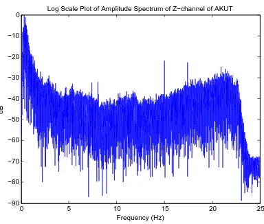
0 5 10 15 20 25 −90
−80 −70 −60 −50 −40 −30 −20 −10
0 Log Scale Plot of Amplitude Spectrum of Z−channel of AKUT
Frequency (Hz)
dB
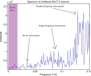
Figure 2.1: The full spectrum for a twenty-minute long signal recorded at station AKUT on an Streckeisen STS-2 broadband seismometer with sampling interval of 0.02 s. Note that the majority of the signal amplitude occurs for frequencies below 2 Hz. This recording was obtained during a seismically quiet time period and therefore includes energy from only the ambient seismic noise sources.
2.3
Spectrum of Ambient Recordings at Akutan
To assess the frequency content of an unfiltered signal recorded at station AKUT, the signal
was Fourier transformed and the amplitude spectrum was plotted. The entire spectrum,
from DC to the Nyquist frequency, is plotted in Figure 2.1.
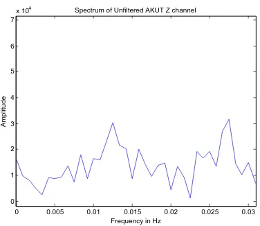
Zooming in on the infragravity frequencies mentioned above, it is found that there is
spectral amplitude for frequencies that are very close to DC. This is in keeping with the
expectations for the frequency spectrum of Earth’s hum (Figure 2.2).
In Figure 2.3, the 26 s microseism is observed. Note that this particular time series was
recorded on August 4, 2008, and therefore one would expect to see that the signal has a
relatively high amplitude when compared to recordings at the same station taken during the
0 0.005 0.01 0.015 0.02 0.025 0.03 0
1 2 3 4 5 6 7
x 104 Spectrum of Unfiltered AKUT Z channel
Frequency in Hz
Amplitude
Figure 2.2: The frequencies from DC to approximately 0.02 Hz are pictured here. Spectral amplitude is found even as one moves towards zero. The very low frequency components of the amplitude spectrum arise from the excitation of lower frequency normal modes by ambient seismic sources.
0.02 0.025 0.03 0.035 0.04 0.045 0.05
0 1 2 3 4 5 6
x 104 Spectrum of Unfiltered AKUT Z channel
Frequency in Hz
Amplitude
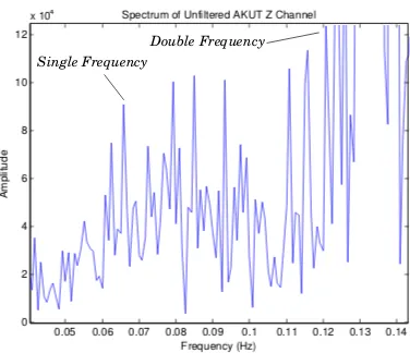
0.05 0.06 0.07 0.08 0.09 0.1 0.11 0.12 0.13 0.14 0
2 4 6 8 10 12
x 104
Frequency (Hz)
Amplitude
Spectrum of Unfiltered AKUT Z Channel
Single Frequency
Double Frequency
Figure 2.4: The single and double frequency microseisms are evident in the plot of the spectrum for the recording at AKUT at approximately 0.06 Hz and 0.12 Hz, respectively. The SF amplitude is less than that of the DF. The lack of a particularly evident individual peak for the two features is in agreement with the relatively broad power spectral density
peaks published elsewhere (see, for example Leeet al., 2011).
Finally, Figure 2.4 shows the primary and secondary multiples for the recording at
station AKUT. The amplitude of the SF is lower than that of the DF, as expected.
To give an idea of the relative amplitude of each of the spectral peaks in the microseism
bandwidth mentioned above, Figure 2.5 shows a closeup of the portion of the bandwidth
that covers the frequencies from the lower range of the Earth’s hum through that of the DF
microseism.
The remaining portion of the spectrum above the DF is undifferentiated strong signal.
In this research, the focus is on frequencies within the portion of the spectrum that has
the largest amplitude, both for each individual recording (as in Figure 2.1), and for the
0 0.05 0.1 0.15 0.5
1 1.5 2 2.5 3 3.5
x 105 Spectrum of Unfiltered AKUT Z channel
Frequency in Hz
Amplitude
Earth Hum
26 sec microseism
Single frequency microseism Double frequency microseism
2.4
Survey Geometry
The IRIS database holds records of time series from several broadband seismometers
sta-tioned on Akutan. The survey geometry is thus imposed: unlike in typical field
applica-tions, there is no opportunity to install and configure array elements in a geometry that
will yield high resolution results. Although the deployment of IRIS instruments in remote
locations and the storage of data has created a wealth of information on current and past
seismic events that is accessible by any interested individual, there exist no current
compre-hensive methods for selecting and interpreting which portions of the recordings should be
used for modeling the subsurface when the only available option is data from a very sparse
and randomly arranged seismic array. This project serves to fill that void.
There are two networks containing broadband instruments that are in use on Akutan.
Data obtained at stations from both will be used in the application of the theories presented
in this dissertation. The first, abbreviated AV for the Alaska Volcano Observatory, is
op-erated by the USGS-Anchorage and the Geophysical Institute at the University of Alaska.
The second network, from which only one station is available, is abbreviated AT for the
Alaska Tsunami Warning Seismic System and is operated by the West Coast and Alaska
Tsunami Warning Center. The broadband recording from the AT network spans the period
from 2002 - present (Incorporated Research Institutions for Seismology, 2012a). There are
13 additional broadband stations in the AT network (≥10 to>80 Hz and corner period
of ≥10 s) spread throughout the southern portion of the state, more than 200 km from
Akutan. The AV network currently has 128 extremely short period (≥80 Hz sampling
rate with corner period of<10 s) seismometers and has had, at various points since 2005,
eight broadband seismometers spread over the island. Unfortunately, only three broadband
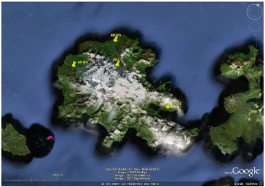
(Incor-Figure 2.6: Stations AKGG, AKLV, AKRB, and AKUT were positioned using the GPS coordinates of each station as recorded in the header of the data files from IRIS.
porated Research Institutions for Seismology, 2012a). The remaining five AV stations are
either unavailable in the database or were online for only very short periods of time. A plot
2.4.1
Selection of Recordings and Data Extraction
Selecting and Retrieving Data from IRIS
Although the available recordings for each network span a number of years in total, there
tend to be gaps in the records at various times and instruments in the networks
through-out the recording periods. The selection of stretches of time where data was recorded at a
maximum number of instruments was desirable so that analysis could be performed with
the largest number of stations for relatively long uninterrupted time series. Because the
goal is to look at microseisms, which are assumed to have periods of 1-10s, only data from
broadband stations were analyzed. The instrument noise for both the Streckeisen STS-2 in
use for the AT network and the Guralp CMG-3T seismometers in the AV network increases
in magnitude at significantly lower periods, on the order of 1000 s citepRinglerHutt2010,
and at frequencies above 10 Hz, so it is assumed that the instrumentation is appropriate
for the frequency ranges of interest. Out of curiosity over the characteristics of signals in
the lower end of the bandwidth of the instruments, analysis proceded for all frequencies of
significantly nonzero amplitude in the power spectra of the broadband recordings at
peri-ods of greater than 1000 s. To determine data availability at each station of interest over a
certain timespan, the index of IRIS data holdings was accessed (Incorporated Research
In-stitutions for Seismology, 2012d). The full description of the IRIS data access and request
procedures may be found in Appendix A. Here, only the details relevant to the extraction
of the specific time series used in this analysis are given.
The IRIS Timeseries Request utility can be used to generate graphs of the data holdings
for a user-defined range of time and stations (or entire networks of stations) to show where
gaps exist in the records of each station over time. Figure 2.7 provides an example of the
AV network.
In this example, it can be seen that gaps exist in the records for several stations. Other
stations, such as AKLV, were apparently turned off for the first or second half of the year
but have full coverage for the times when they were in use. The search format described
in Appendix A, Section A.2, can be used to generate a graph for the network and time
period of choice, up to one year in duration. Time ranges longer than one year apparently
overwhelm the plotting capabilities of the system.
To obtain data for this project, a bounding box search (see Appendix A) was conducted
over the island of Akutan to determine which stations were available. The graphic display
from the Timeseries Request utility was used to find stretches of time with the best
cover-age. Out of all of the instruments at the AV network, three broadband stations were found
to have long, uninterrupted recordings in the years 2005, 2008, and 2009. A fourth station
in the AT network also had decent coverage in these years. A breq fast request,
formu-lated as detailed in Section A.5 of Appendix A, was then sent to IRIS to obtain the seismic
record in the SEED format for these stations over a period from May 16, 2008 to February
16, 2009. This stretch of time was chosen for two reasons: first, it covers both summer
and winter conditions. Second, all four stations were recording for the majority of the time
AV.AKRB.*.*(100.0%)
AV.AUW.*.*(100.0%) AV.AUL.*.*(91.2% - 3 gaps) AV.AUH.*.*(87.9% - 2 gaps)
AV.BGR.*.*(100.0%) AV.ANON.*.*(75.7%- 1 gap)
AV.CETU.*.*(76.2%- 1 gap) AV.ADAG.*.*(52.7% - 3 gaps)
AV.BRPK.*.*(100.0%)
AV.CERB.*.*(81.0%- 1 gap) AV.BLHA.*.*(100.0%) AV.AKV.*.*(100.0%) AV.BGM.*.*(100.0%) AV.AKS.*.*(100.0%) AV.CDD.*.*(100.0%) AV.BPBC.*.*(100.0%) AV.AKGG.*.*(100.0%)
AV.CEPE.*.*(72.7%- 1 gap) AV.AUE.*.*(76.8%- 1 gap)
AV.CGL.*.*(100.0%) AV.ANNW.*.*(100.0%) AV.AHB.*.*(100.0%)
AV.CERA.*.*(90.9%- 1 gap) AV.CEAP.*.*(81.0%- 1 gap) AV.BGL.*.*(100.0%) AV.AUNW.*.*(100.0%) AV.AUP.*.*(100.0%) AV.ANPK.*.*(75.1%- 1 gap) AV.ANNE.*.*(75.7%- 1 gap)
AV.AUI.*.*(76.8%- 1 gap) AV.ANPB.*.*(75.7%- 1 gap)
AV.BKG.*.*(100.0%) AV.BLDY.*.*(100.0%) AV.AKLV.*.*(100.0%)
AV.CESW.*.*(76.2%- 1 gap) AV.AMKA.*.*(92.2% - 10 gaps) AV.ACH.*.*(100.0%) AV.AZAC.*.*(100.0%) AV.ANCK.*.*(100.0%) AV.CAHL.*.*(100.0%) 2009 01-01 06:00 2009 03-01 00:00 2009 05-01 00:00 2009 07-01 00:00 2009 09-01 00:00 2009 11-01 00:00 2010 01-01 12:00 2010 03-01 12:00 Date/Time
Waveform Data By Day Quality=ALL for AV, *, *, * Time Spans and Percent
Percent by First/Last Time Range (Average = 91.4%)
Overlap
Continuous
Gap
(a) (b)
Chapter 3
AMBIENT SEISMIC NOISE METHODS: AN
HISTORICAL PERSPECTIVE OF STATISTICAL
TECHNIQUES
3.1
On the Origin of the Term “Ambient Seismic Noise,”
Consideration of Its Source, and Its Applications
Microtremors, sometimes also called microseisms, are the constant low amplitude
vibra-tions of the earth’s surface and include both body and surface waves (Okada, 2003). The
amount of dispacement of the surface from microtremors is far below human perception,
and yet the vibrations remain a source of noise in earthquake studies. Especially when
trying to study very distant or small earthquakes, microseisms often obscure the desired
signal as their amplitude increases whenever amplifier gain is increased. One of the main
focuses of earthquake seismology research through the 1970s was the removal of the
mi-croseism signal from the earthquake signal. In this way, the phenomenon has earned the
The “ambient” portion of the term is used to convey the pervasive nature and lack of
impulsive source for the signal — ambient seismic noise has been observed at stations
all around the world, and possible origins include anthropogenic sources, such as ship or
foot traffic, motion of water in waves in the oceans and rivers, and changes in atmospheric
pressure. In the literature, many researchers focus on using ambient seismic noise data
for the calculation of subsurface velocity profiles. For these studies, the source of ambient
seismic noise is always considered to be diffuse. However, as was discussed in Chapter 2,
there is an entire body of work devoted to determining whence the ambient signals arrive
and discussing the implications of the temporal and spatial variations in the source. That is,
rather than considering only omnidirectional and pervasive noise, there is insteadalways
a source and it is likely that the source may be highly directional. The work presented
here differs distinctly from the usual assumption that any one station used as the first term
in a cross correlation to compare the waveforms at two stations within an array can serve
as a virtual source because the ambient energy is coming from all directions at all times.
Here, it is assumed that there is an actual source of the noise and that energy does not
necessarily always arrive from all azimuths. For this case, it is crucial to understand which
array elements are closest to the actual source in order to correctly determine travel times
and, thus, velocity structure.
In recent times, the advent of digital recording and increased capacity of data storage
media has made feasible the interpretation of ambient noise for subsurface exploration.
Sta-tistical analysis of microtremor has proven that the noise is generally a stationary stochastic
process. In Okada (2003), a review of the methods of analysis is provided. It was found
that, regardless of time, the microtremor signal for signals lasting less than three hours
ampli-tude, implying that the microtremor signal is a stationary stochastic process. However, it
was also observed that the stationarity did not hold for signals measured more than three
hours apart from each other. Stationarity in space has also been observed over distances
of 1-3 km. Beyond this distance, it appears that the stationarity in space is assumed rather
than proven. A particular advantage of the work presented in this dissertation is that the
as-sumption of stationarity in space and time is unnecessary as the method is equally capable
of handling non-stationary, non-stochastic, and highly directional signals. Once the noise
was proven to be stationary in time (when measured over appropriate lengths of time) and
space (over limited volumes) and could be represented as a stationary stochastic process,
one of two primary statistical methods of detecting the surface waves in the noise is
typ-ically applied, depending on the survey geometry. The first is the spatial autocorrelation
coefficient method by Aki (1957). The second is the frequency-wavenumber (f-k) method.
The f-k method uses only the signal measured by the vertical component of the seismometer
or geophone and, by the assumption that surface waves dominate the body waves recorded
as microseismic noise, only measures Rayleigh waves. The SPAC method is also capable
of using information from the horizontal channels and can thus analyze Love waves if they
arise (Okada, 2003). The number of studies that use one of these two methods to produce
images of the subsurface from recordings of the noise signal at two or more stations has
in-creased dramatically since the first successful studies by Okadaet al.(1990), Shapiroet al.
(2005), and Sabraet al.(2005). Although each method has its advantages, disadvantages
also exist that limit the feasibility of using seismic noise data in particular circumstances
as described in Sections 3.2 and 3.3 below.
For the case of Akutan, even without the assumption of directional noise, it is apparent
on the island. It is the pursuit of using seismic noise for determining velocity models of the
subsurface for both arrays and recording times that are unsuitable for either method that
forms the motivation of this study.
3.2
Spatial Autocorrelation Coefficient Method
One of the earliest and most commonly cited publications on the stationary stochastic
nature of ambient seismic noise and the possibilities for attainment of dispersion curves
thereof comes from Aki (1957), where the stochastic method now known as the spatial
au-tocorrelation coefficient (SPAC) technique was first explored in detail. The paper attempts
to provide a method of analysis for time and space spectra of seismic noise where it is
too complicated to perform phase analyses. This is the earliest example in the literature of
representing both the temporal and spatial components of microseismic noise as stationary
stochastic processes. The product of this investigation was the first step towards a
solu-tion to the problem of pervasive microtremor noise in seismic signals found in recordings
made with the intent of detecting earthquakes in Japan that reveals the statistical character
of the noise as well as the subsurface through which it travels via the production of phase
velocity dispersion curves. The investigation of microtremor noise was motivated by the
study by Kanaiet al.(1954), among others, where it was observed that the spectral peaks
for microtremor noise were identical to those produced by earthquakes and were affected
by the local geology where the signal was observed. Unfortunately, due to the lack of
digital recording methods, the analysis of signals with frequencies above 1 Hz and the
at-tempt to determine the phase velocity curves was unsuccessful because the signals were
not stationary over the limited length of time that they could be recorded.
as the method is not used for analysis, but a rough outline is provided in Appendix D,
Section D.2, to inform the discussion of the limits of the method for the particular case of
the array at Akutan.
From the outline of the derivation in Appendix D, it is obvious that the method of
SPAC is unconcerned with determining the source direction of the noise since the results
arise from spatial averaging of signals from all angles. Instead, the SPAC method seeks
to find the scalar velocity of the signal. The technique is only viable for omnidirectional
sources of noise due to the requirement of a circular or, at the least, a particularly precise
array of three sensors at the points of an equilateral triangle and one sensor located at its
center (Okada, 2003), and the spatial autocorrelation coefficient itself is a function of the
array radius as well as the frequency and phase velocity.
One of the primary benefits of the SPAC method as compared to the f-k method
dis-cussed in the next section is that the array size required for SPAC is much smaller and
requires fewer components. The method also allows one to observe Love waves in addition
to Rayleigh waves if three component seismometers or geophones are used. The ability
to isolate the Love wave signal and the simplicity of extending the Rayleigh wave
the-ory to the case of Love waves is particularly attractive because it allows one to determine
the s-wave velocity model for the subsurface, which is not possible when using the f-k
method (Okada, 2003). Aki’s 1957 suggestions for applications for microtemor analysis
included locating the source of volcanic tremor, studying the coda of waves generated in
earthquakes, and discovering the location of the epicenter for small earthquakes. In light
of the research suggesting that many components of the ambient seismic spectrum are not
homogeneously distributed (see, for example, the references in Chapter 2), the SPAC
this technique.
Subsequent to the publication of the paper by Aki in 1957, the field of research
involv-ing SPAC was mostly limited to studies in Japan as scientists in the west focused more on
finding the direction of energy, possibly due to a desire to locate signals within the
micro-seism bandwidth generated by nuclear tests during the Cold War, and limits in the amounts
of data that could be recorded prevented the collection of stationary data sets. Even in
recent years, the requirements for specific survey geometry limits the number of cases in
which SPAC can be applied. Several studies do exist, however. Besides the examples cited
in the SEG monograph by Okada (2003), other studies have since come to completion (e.g.,
Haneyet al., 2012). It is difficult to overstate the influence of Aki’s seminal publication in
convincing scientists of the potential for using rather than attempting to eliminate seismic
noise.
3.3
Frequency-Wavenumber Spectral Method and
Beam-forming
The power spectrum of a random time series is a description of the frequency content of
that signal. The expansion of this concept to a series that is also stationary in space requires
the addition of a spatial dimension to the power spectrum, as well. This new spectrum is
the frequency-wavenumber (f-k) spectrum, also referred to as the frequency-wavenumber
power spectral density (PSD). The information contained in the f-k PSD describes, in the
case of signals consisting of spatially and temporally stochastic microseismic noise, both
the frequency content and the vector velocity of the signal. The f-k spectrum is thus a
velocity of a high-energy signal in the microtremor bandwidth. As in the SPAC method, the
information used to build dispersion curves comes from the spectra of the signals received.
Velocity models of the subsurface may be produced by inversion of either phase- or
group-velocity dispersion curves.
Historically, the theory for the f-k technique was first developed and then applied during
the Cold War because of its suitability for detecting the directional component of the
veloc-ity vector of waves generated by underground nuclear testing (Okada, 2003; Capon, 1969).
The focus on the direction of arrival is the most elemental difference in the functionality
of the SPAC and f-k methods. Other significant differences between the two methods
con-cern the type of energy that the method is capable of measuring and the requirements for
array geometry. Although one may assume that the majority of the wave energy in the
mi-croseismic signal comes from surface waves, the f-k method does not discriminate against
strong signals from body waves. Researchers may opt to use only the vertical component
of a sensor to focus on Rayleigh waves. Like the SPAC method, the array size for the f-k
method is chosen based on the depth to the target of interest. Although the requirements
for survey geometry are much less specific for the f-k method, resolution of vector velocity
increases with the number of array elements because larger arrays contain larger numbers
of station pairs.
There are two ways of determining the f-k power spectrum for a signal that may or may
not be a stochastic process. The first way consists of executing the normal steps used to
find the frequency-only power spectral density of a time signal — find the autocorrelation
function, then apply a Fourier transform to it — but for a signal with both a time and
space component. The second way consists of first applying a finite Fourier transform or