University of New Orleans University of New Orleans
ScholarWorks@UNO
ScholarWorks@UNO
University of New Orleans Theses and
Dissertations Dissertations and Theses
Spring 5-16-2014
A Multivariable Statistical Approach to Managing United States
A Multivariable Statistical Approach to Managing United States
Coast Guard Small Boats
Coast Guard Small Boats
Brian D. Fitzpatrick
University of New Orleans, bdfitzpa@uno.edu
Follow this and additional works at: https://scholarworks.uno.edu/td
Part of the Operations Research, Systems Engineering and Industrial Engineering Commons
Recommended Citation Recommended Citation
Fitzpatrick, Brian D., "A Multivariable Statistical Approach to Managing United States Coast Guard Small Boats" (2014). University of New Orleans Theses and Dissertations. 1797.
https://scholarworks.uno.edu/td/1797
This Thesis-Restricted is protected by copyright and/or related rights. It has been brought to you by
ScholarWorks@UNO with permission from the rights-holder(s). You are free to use this Thesis-Restricted in any way that is permitted by the copyright and related rights legislation that applies to your use. For other uses you need to obtain permission from the rights-holder(s) directly, unless additional rights are indicated by a Creative Commons license in the record and/or on the work itself.
A Multivariable Statistical Approach to Managing United States Coast Guard
Small Boats
A Thesis
Submitted to the Graduate Faculty of the
University of New Orleans
in partial fulfillment of
the requirements for the degree of
Master of Science
in
Engineering Management
by
LT Brian D. Fitzpatrick, USCG
B.S. United States Merchant Marine Academy, 2005
ii
iii
Acknowledgement
The author would like to acknowledge the Office of Naval Engineering CG-45, Surface Forces Logistics Center, and the following people for their contribution to this research: CDR Scott Keister, Mr. Randy Gardner, LCDR Matthew Hammond, Mrs. Luanna Straker, Dr. George Parakevopoulos and the rest of the Small Boat Product Line. Without these dedicated people and organizations this research would have never been possible.
iv
Table of Contents
List of Tables ... vi
List of Figures ... vii
List of Acronyms ... viii
Abstract ... ix
Chapter 1: Introduction ... 1
United States Coast Guard Coast Guard ... 1
USCG Logistics System Overview ... 1
Surface Forces Logistics Center-Small Boat Product Line Organization ... 2
Small Boat Operations ... 4
Performance Measures ... 4
Chapter 2: Literature Review ... 6
Calculation of Asset Operational Availability ... 6
Process Control ... 7
Normal Distribution ... 8
Bivariate Normal Distribution ... 8
Expected Value ... 10
Forecasting Models ... 10
Maintenance Cost per Operating Hour ... 11
Small Boat Allocation Optimization ... 12
Chapter 3: Methodology ... 13
Monthly Seasonal Index ... 13
Two Dimension Regressions ... 14
Statistical Process Control and Normal Distribution ... 15
Linking Monthly Data to Derive Curve ... 15
Expected Value ... 16
Models Resulting From a Mandate to Increase Operational Availability ... 17
Lifecycle Cost Estimates ... 17
v
Statistical Process Control ... 19
Cost Versus Operating Hours ... 22
Cost versus Operational Availability ... 24
Multi-Regression of Cost as a function of Operational Availability and Operating Hours ... 26
Bivariate Normal Distribution ... 27
Expected Cost ... 28
Lifecycle Cost Estimate ... 29
Chapter 5: 47 MLB Results ... 30
Statistical Process Control ... 30
Cost Versus Operating Hours ... 33
Cost versus Operational Availability ... 34
Multi-Regression of Cost as a Function of Operational Availability and Operating Hours ... 35
Bivariate Normal Distribution ... 37
Expected Value ... 38
Lifecycle Cost Estimate ... 38
Chapter 6: Recommendations ... 38
Use of Statistical Process Control ... 38
Unify the Information Technology System ... 39
Management Track on a Monthly Basis ... 39
Managing Operational Availability ... 40
Develop New Metric ... 40
Maintenance Cost per Availability Hour ... 41
Continuing Training ... 42
Chapter 7: Conclusion ... 44
Works Cited ... 45
Appendix A: 25 RB-S Multivariable Regression Data ... 47
Appendix B: 47 MLB Multivariable Regression Data ... 49
Appendix C: 25 RB-S Expected Value Calculations ... 50
Appendix D: 47 MLB Expected Value Calculations ... 51
vi
List of Tables
Table 1: Seasonal Index for 25 RB-S ... 14
Table 2: Seasonal Index for 47 MLB ... 14
Table 3: 25 RB-S Projected Availability Models ... 17
Table 4: 47 MLB Projected Availability Models ... 17
Table 5: 25 RB-S Sensitivity Analysis ... 27
Table 6: 25 RB-S Operational Availability Models ... 28
Table 7: 25 RB-S Estimated Total Lifecycle Cost ... 29
Table 8: 47 MLB Sensitivity Analysis ... 36
Table 9: 47 MLB Calculated Expected Value ... 38
vii
List of Figures
Figure 1: SFLC Small Boat Product Line Organization ... 3
Figure 2: 25 RB-S Operational Availability Control Chart ... 19
Figure 3: 25 RB-S Operational Availability Histogram ... 20
Figure 4: 25 RB-S Operating Hours Control Chart ... 21
Figure 5: 25 RB-S Operating Hours Histogram ... 22
Figure 6: 25 RB-S Cost versus Operating Hours ... 23
Figure 7: 25 RB-S Operating Hours versus Cost ... 24
Figure 8: 25 RB-S Total Cost vs Operational Availability ... 25
Figure 9: 3-D Plot of Cost as a function of Operational Availability and Operating Hours ... 26
Figure 10: 25 RB-S Bivariate Normal Distribution Graph ... 27
Figure 11: 47 MLB Operational Availability Control Chart ... 30
Figure 12: 47 MLB Operational Availability Histogram ... 31
Figure 13: 47 MLB Operating Hours Control Chart ... 32
Figure 14: 47 MLB Operating Hours Histogram ... 33
Figure 15: 47 MLB Cost versus Operating Hours ... 34
Figure 16: 47 MLB Cost versus Operational Availability ... 35
Figure 17: 47 MLB 3-D Scatter Plot of Cost as a function of Hours and Availability ... 36
viii
List of Acronyms
25 RB-S – 25 FT Response Boat Small47 MLB – 47 FT Motor Life Boat
Ao – Asset Operational Availability
CG-LIMS – Coast Guard Logistics Information Management System
DCMS – Deputy Commandant for Mission Support
DHS – Department of Homeland Security
DOD – Department of Defense
EAL – Electronic Asset Log
FLS – Fleet Logistics System
FMC – Fully Mission Capable
IT – Information Technology
NMCD – Not Mission Capable Depot
NMCL – Not Mission Capable Lay-up
NMCM – Not Mission Capable Maintenance
NMCS – Not Mission Capable Supply
pdf – Probability Density Function
PL – Product Line Generic
PMC – Partially Mission Capable
PWCS – Port, Waterways, and Coastal Security
SAR – Search and Rescue
SBPL – Small Boat Product Line
SFLC – Surface Forces Logistics Center
ix
Abstract
The Coast Guard has developed several systems to measure the performance of its engineering and logistics
organizations. The development of these measures is based upon the need to show where and how
the organization meets the American taxpayer’s needs. The use of multivariable regressions and
determining the statistical distributions of the variables will show the adequacy of the measures and
processes currently used. They will also determine a better way to measure the performance of the
Coast Guard Small Boat Fleet. This research will analyze the 47 Motor Life Boat and
25 Response Boat-Small data from fiscal year 2011 to 2013. The focus will be on improving the
measure used by the engineering and systems managers of the Coast Guard to manage assets and resources,
as well as making recommendations on how to improve the processes involved in managing a robust
engineering and logistics system.
1
Chapter 1: Introduction
United States Coast Guard Coast Guard
The United States Coast Guard is one of the five services of the United States Military, and is the only service outside of the Department of Defense that resides within the Department of Homeland Security. The Coast Guard was founded in 1790 as the Revenue Cutter Service, and has evolved into a large multi-mission maritime service that includes the U.S. Lifesaving Service, U.S. Light House Service, Steamboat Inspection Service and other former federal agencies. The Coast Guard’s missions have remained relatively consistent since 1915, when the Revenue Cutter Service merged with the U.S. Lifesaving Service, becoming today’s Coast Guard. The Coast Guard has 42,000 Active Duty Members, 8,000 Reservists and 8,800 Civilian employees that support 11 statutory missions: Port, Waterways and Coastal Security; Search and Rescue; Ice Operations; Drug Interdiction; Aids to Navigation; Living Marine Resources; Marine Safety; Defense Readiness; Migrant Interdiction; Environmental Protection; and other Maritime Law Enforcement missions. The Coast Guard operates a variety of aircraft, ships and small boats as part of its inventory to complete its diverse mission set, and each platform has a myriad of primary and secondary missions it can perform. Operating with a total annual budget of $8.1 billion, the Coast Guard has a total of 210 aircraft, 244 ships (or cutters) and 1,800 small boats. (United States Coast Guard)
The Coast Guard’s headquarters is organized into two large directorates. The first is the Deputy Commandant for Operations (DCO), which oversees all operations and operations policy including how and where search and rescue is performed, interactions with combatant commands of Department of Defense, how ships are inspected and how mariners are licensed. The second directorate is the Deputy Commandant for Mission support that provides all personnel support, training, Command, Control, Communications, Computers, and Information Technology (C4IT), engineering and logistics, and acquisitions to support all of the DCO’s missions. These two deputy commandants oversee the top-level executives in the Coast Guard for each area. The individual deputy commandant oversees the policy for which he or she is responsible. This provides the span of control necessary to operate a large, complex government organization with a variety of mission sets.
USCG Logistics System Overview
The U.S. Coast Guard’s logistics model is based on four essential pillars of logistics combining a product line management, Bi-Level Maintenance, Total Asset Visibility and Configuration Management. The Deputy Commandant for Mission Support (DCMS) defines each of these at the enterprise level. The logistics system supports all of the Coast Guard’s assets including aircraft, small boats, ships, installations and personnel. The system is broken down into several directorates, Commands and product lines, with the ultimate goal of providing “sustained and adequate readiness to all Coast Guard mission.” (Currier, 2010)
2
The Bi-level maintenance model is broken into two categories — organizational level and depot level. The organizational level is completed by personnel at the specific station for a particular boat. The depot level is completed by the involvement of the specific product line responsible for the asset.
Total asset visibility creates transparency between the operational unit and the product line. This is achieved by the use of live databases to communicate asset statuses. The asset statuses are recorded, and this becomes the raw data for everything including crew, boat and maintenance hours. The system also allows operational units to communicate asset casualties and check the status of parts orders and upcoming maintenance.
Configuration management allows for mass purchases of parts and materials by the specific product line for a specific asset. A standard configuration also allows the quick transfer of the asset to a new or different station — the crew will know the operating characteristics and equipment locations or functions of the boat. This allows for rapid re-deployment of both assets and personnel, and also reduces training costs. (Currier, 2010)
The concepts for the four cornerstones of logistics are generally applied principles of total quality management. The Coast Guard’s aviation community was the first to adapt to concepts in support of fixed and rotary wing aircraft. The four pillars of logistics provide for a high-level business blueprint for all Coast Guard Logistics organizations under the DCMS. The mission support system provides support for all personnel and assets including human resources, training, electronics, information technology, logistics, engineering and acquisitions. Each segment of mission support operations has its own directorate within the Coast Guard headquarters organization.
Surface Forces Logistics Center-Small Boat Product Line Organization
Figure 1: SFLC Small Boat Product Line
The Engineering Branch is sub
provide maintenance and lifecycle management of specific assigned assets. The Systems Equipment Specialist Section provides propulsion and elect
Maintenance System Section provides data integrity in the maintenance system. The three other sections are the asset management sections that provide engineering and logistics support to the fleet and responsible of the lifecycle management of the assigned assets. Often the asset management sections are comparatively “Mini-Product Line Managers” in their scope of
The Planned Depot Maintenance Branch (PDM) is respon execution of the depot maintenance for those assets requir
two sections — one for each the E and guidelines.
The Supply Branch is divided into three sections that cover three different assigned duties. The first is the inventory management section,
delivered, and shipped to the various units. The eq
repairable items and works in conjunction with the inventory managers to ensure the inventory is packaged and delivered properly. The financial section maintains the financial recor
product line. (Keister, Small Boat Product Line Standard Operating Procedure, 2011)
3 : SFLC Small Boat Product Line Organization
The Engineering Branch is sub-divided into five sections that support heavy technical analysis or provide maintenance and lifecycle management of specific assigned assets. The Systems Equipment Specialist Section provides propulsion and electronics technical support, while the Asset Computerized Maintenance System Section provides data integrity in the maintenance system. The three other sections are the asset management sections that provide engineering and logistics support to the fleet and responsible of the lifecycle management of the assigned assets. Often the asset management sections are
Product Line Managers” in their scope of responsibilities and duties.
The Planned Depot Maintenance Branch (PDM) is responsible for the scheduling, planning, and execution of the depot maintenance for those assets requiring depot maintenance. The Branch is split into East Coast and West Coast — that follow the same business structure
The Supply Branch is divided into three sections that cover three different assigned duties. The first is the inventory management section, which specifically ensures that inventory is purchased, delivered, and shipped to the various units. The equipment specialist section develops repair contracts for repairable items and works in conjunction with the inventory managers to ensure the inventory is packaged and delivered properly. The financial section maintains the financial recor
(Keister, Small Boat Product Line Standard Operating Procedure, 2011)
divided into five sections that support heavy technical analysis or provide maintenance and lifecycle management of specific assigned assets. The Systems Equipment while the Asset Computerized Maintenance System Section provides data integrity in the maintenance system. The three other sections are the asset management sections that provide engineering and logistics support to the fleet and are responsible of the lifecycle management of the assigned assets. Often the asset management sections are
responsibilities and duties.
sible for the scheduling, planning, and depot maintenance. The Branch is split into that follow the same business structure
4
Small Boat Operations
The Coast Guard has 188 small boat stations located throughout the continental United States, Alaska, Hawaii, and territories. These multi-mission stations perform or support each of the Coast Guard’s 11 statutory missions. Stations maintain several capabilities for both inshore and offshore response efforts. Each station has a variety of platforms with several different combinations depending on the area of responsibility. Two of the most populous platforms in the Coast Guard inventory are the 25’Response Boat-Small “Defender” A/B Class (25 RB-S) and the 47 FT Motor Life Boat (47 MLB). These two platforms perform all of the Coast Guard’s missions and play a key role in the execution of the tactical and strategic missions of the Coast Guard.
The 25 RB-S is a 25-foot semi-planning hull with cabin and two 225 horsepower Honda outboard engines. The boats were constructed by Safe Boats International from 2002 to 2009. The 25 RB-S was built in response to the September 11 terrorist attacks in order to provide the Coast Guard a standard response boat to preform SAR and PWCS missions. The Coast Guard currently operates 400 at Stations, Marine Safety and Security Teams (MSST), and Marine Safety Units, and is the largest boat class in inventory. (United States Coast Guard)
The 47 MLB is a 47-foot self-righting hull with two inboard Detroit Diesel 6v92 engines constructed by Textron Marine and Land Systems from 1995 to 2003. (Textron Marine and Land Systems) The platform’s unique capability to right itself in an intact stability condition makes it best for heavy surf conditions. There are 117 47 MLBs in service and perform SAR missions in breaking surf and heavy weather as well as offshore. 47 MLB’s are only operated from Stations. (United States Coast Guard)
Stations operate as independent units directed by a central tactical command called a Sector, which is also the parent unit of the station. Each station operates and performs organizational level maintenance on its own boats with some limited assistance from the Sector. Stations range in size based on location operating level and prevailing weather conditions in the geographic area. This also determines the station’s allowance of boats. Therefore, Station New York is a significantly larger unit with more boats and personnel than Station Ludington in Michigan, because of the need to protect New York harbor and provide search and rescue operations in that heavily trafficked port. Sectors provide engineering and logistics support in the form of maintaining parts inventories and engineering sections that can augment the station crews. Stations have a 24- hour duty section, or crew. This varies between stations with the number of boats, personnel, and operational requirements of each station. (Krietemeyer, 2000)
Performance Measures
5
available for operations to the tactical commander. The tactical commander cares solely about having the correct boat, aircraft, or ship available to respond to the mission. The final measure that is incorporated into all parts of the decision-making process is the amount of funding required to accomplish the needs of the individual measure. The funding level expended can be used as a measure or indicator.
At some level, these measures all have an effect on one another. Such a chain could be established that would show that if an asset was not operationally available during a period of time, the asset would not perform any operational hours, and therefore not be able to save a life or interdict illicit drugs. As can easily be deduced, the chain of variables have a cost that must be expended to maintain the assets.
6
Chapter 2: Literature Review
Calculation of Asset Operational Availability
Asset operational availability (Ao) is a probability function showing the reliability, maintainability, and supportability of the system. (Moore, 2003) The data for input is tracked in Electronic Asset Log (EAL) as the small boat stations change the status of the boats from several different statuses. The statuses are tracked based on a length of time and then converted into probabilities. The USCG partially departs from the U.S. Navy’s terminology when considering the statuses. The statuses outlined in the SBPL Standard Operating Procedure in the drop down menu are as follows:
• Fully Mission Capable (FMC) – the boat is ready for all assigned missions in every respect. • Partially Mission Capable (PMC) – the boat is ready for certain missions however has a casualty
that will prevent it from completing a specified task. Example: 25 RB-S Aft passenger seat is in-operable, the boat can get underway without any issue however no one can sit in one of the aft passenger seats.
• Not Mission Capable Supply (NMCS) – The boat is awaiting supplies or a parts order to be repaired, in this state the boat is not able to get underway and is not available for operations. • Not Mission Capable Maintenance (NMCM) – The boat is undergoing organizational level
scheduled maintenance or organizational level repair.
• Not Mission Capable Depot Maintenance (NMCD) – The boat is undergoing scheduled or unscheduled depot maintenance availability. The 47 MLB has four year scheduled maintenance availability, the 25 RB-S does not.
• Not Mission Capable Lay-up (NMCL) – The boat is in a lay-up status for seasonal reasons, decommissioning, or transfer to another unit. In cold climates that accumulate ice, such as the Great Lakes, the Coast Guard winterizes all small boats and places them in a lay-up status.
Most notably, the departure by the USCG from the Navy is with Mean time between failure, which is the sum of PMC and FMC. Mean time to repair is the sum of NMCM and NMCD. Mean logistics delay time and NMCS are equivalent. This change in terminology is to meet the operational nature of EAL — it would be hard for an operational unit to describe a boat being in the mean time between failure and the boat is ready for operations. These EAL statuses are monitored daily by the SBPL, Sector Engineers, and Sector or District Command Centers. The information provided in the status updates give a quick snap shot of the availability at a particular unit. The statuses are updated real time in the system and then recorded in the memory of the system.
SBPL then converts the periods of time into probabilities by dividing the sum of each status total by the total time available for the asset class. Availability as defined by OPNAVINST 3000.12A is “a measure of the degree to which an item is in an operable and committable state at the start of a mission when the mission is called for at an unknown (random) point in time.” The mathematical definitions are as follows for each probability:
∑
7
∑
∑ ∑
∑
∑
∑ ∑
∑
The mathematical definition of Ao:
∑
∑
1
*Note: NMCL is dropped from all calculations as the boat is in a special status
The Ao figures are calculated once a month for each asset class and as an overall average for the entire boat fleet. The current target for Ao is 80%, for each class with a SAR requirement. Both the 47 MLB and 25 RB-S are SAR vessels and at units that have a SAR mission requirement. Recent changes in the small boat fleet due to the Coast Guards Boat Optimization initiative potentially have changed the Ao target for the 47 MLB and 25 RB-S due to the elimination of spare assets in areas. The SBPL expects the requirement to increase Ao to a new target of 85% Ao, while maintaining comparable levels of operating hours. (Keister, Small Boat Product Line Manager, 2013)
Process Control
8
∑
!! " #"$ % 1
1 & $
'
()*
Using good general management practice, the control limits were calculated by using three standard deviations. The data appeared to fit a normal distribution for both operational availability and operating hours when put into a histogram.
+!!" , 3 . "
Having calculated the upper and lower control limit, the next three fiscal years were plotted on the control chart. For each asset class, the control charts were then used to determine if the asset was within statistical control or had fallen out of statistical control. To determine statistical control, one must look at each data point to determine if it is between the upper and lower control limit and look for trends in the data itself. If the data moves within the control limits in a trend for a number of periods, the system is out of control. The data set that moves randomly within the control limits is in statistical control. There are allowances for seasonality, as certain products are seasonal in nature and will have natural tendencies to behave with a high season and a low season, so they may not appear as random as a product that is not seasonal. (Heizer, 2008)
Normal Distribution
The normal distribution is often used in manufacturing and management as it is a distribution that is often naturally occurring with random variables. (Devoure, 2000) The assumption that will need to be proven in the analysis will be that the variables of operational availability and operating hours fit or closely fit the description of a normal distribution. Mathematically, the normal distribution is defined as the probability distribution function:
/ 1
√22 3
45647$89 :9
, ∞ = = ∞
This will be applied to the distribution of the actual variable graphed in a histogram for the period being evaluated. The resulting plot will show the continuous function of the normal distribution over the interval covered by the histogram. (Hogg, 2010) When the assumption is proven true, the variables of operational availability and operating hours will be treated as random variables with a normal distribution throughout the rest of the analysis.
Bivariate Normal Distribution
9
turns into the volume of the area under the curve verse the area under the curve as is the basis of the normal distribution or any other two dimensional distribution.
The Bivariate Normal Distribution accounts for the covariance in the expected value of the two random variables used in calculating the pdf. The covariance of two random variables is calculated using the standard deviation of the two random variables and the correlation coefficient, or stated mathematically:
>, ? @3x3Y @ ! //!A!
The useful portion of this when deriving the pdf of the bivariate normal distribution is the correlation coefficient. This describes the relationship between the X and Y random variables. The correlation coefficient falls between negative one and one, and when equal to zero, the random variables X and Y are said to be independent. (Hogg, 2010)
1 = @ = 1
@ 0, > ? C D E!F"
The bivariate distribution for independent variables is quite simple and one could expect with the correlation coefficient equal to zero.
/>, ? 1
223X3Y#1 @$
4*$ 5GH478XxI
9 JGH47Y
8Y I
9 :
When X and Y are not independent, the equation is essentially the same. However, the correlation coefficient appears as it is not equal to zero and adds to the equation.
/>, ? 1 223X3Y#1 @$
*4K5G* H478XxI
9
4$KGH47x
8X IGL47 Y
8Y IJGL47 Y
8Y I
9 :
This is also known as the bivariate normal distribution. Just like a two-dimensional pdf, the resulting three-dimensional pdf will be equal to one from X and Y negative infinity to positive infinity. (Hogg, 2010) The analysis will have to calculate the correlation coefficient in order to determine which form of the bivariate normal distribution to use. The bivariate normal distribution when evaluated between negative infinity and infinity for both X and Y.
1 M M />, ? NO
4O O
10
Expected Value
The expected value of a probability function is simply the product of the utility function and the probability function. When dealing with continuous probability functions it becomes the integral of the product of the probability density function (pdf) and the utility function or mathematically:
P> M Q/ O
4O
With
/ / Q Q!!N /QA!
By definition, the expected value is equal to the mean of the distribution. The expected value combines the probability and the value of the utility function. The expected value will be applied in the business sense as the expected profit of the decision. In the case of a government or non-profit organization, avoiding or reducing cost is the basis. In this analysis, the reduction of cost is the basis, so selection of the least cost will be utilized.
Expected value of the bivariate is calculated similarly to the expected value of a single variable. Thus the mathematical equation is:
P, R M M , R/, RR
With,
, R A" S""!
/, R T! ! !"!FQ! / " " /QA! / R
Forecasting Models
Business forecasting models are based on data point collected to project the next period’s sales, earnings, amount to manufacture or other measure. The objective is to determine how much to produce, purchase, or sell. The Coast Guard and the SBPL are not profit-making organizations, but can still use some of the same principles to develop decision models. The objective of forecasting is to predict the future demand or production of a system. In this sense, the system produces both Ao and operating hours. The study will evaluate each of the product data sets, operational availability and operating hours, to provide estimates of the individual outputs throughout the year.
11
parameters weather in the northern half of the country, and reduced numbers of shipping and recreational boating during these periods. To calculate the seasonal indexes for the classes followed the below process:
" C U W VN SVN S
This monthly forecast will be compared to the actual produced in the month. The SBPL or SFLC do not have control of the number of operating hours completed by the operational units because they are under the control of USCG Districts and Sectors. However, operating hours have a direct relationship with cost that can easily be explained.
Maintenance Cost per Operating Hour
Maintenance Cost per Operating Hour is a measure currently used for all surface assets by the SFLC. The measure is a simple linear function that shows the relationship between cost and operating levels. Current SFLC policy is to calculate and publish the Maintenance Cost per Operating Hour (MCPOH) on an annual basis. The SBPL has been able to calculate MCPOH for the past three years using the data collected from the various fleet information systems including Asset Logistics Information System (ALMIS), Fleet Logistics System (FLS), and Abstract of Operations System (AOPS). The calculation is based on the average boat of each boat class.
The MCPOH formula used by the SBPL is as follows:
WR Σ S W!S RQ" F ! A""Σ S " F ! A""
Σ S " F ! A"" QF / T" ! ""ΣQ P!Q"
Σ S W!S RQ" T ! "" ΣQ W!S RQ"QF / T" ! ""
12
Small Boat Allocation Optimization
The study of asset allocation and the size of the small boat fleet has always been a discussion within the Coast Guard and the subject of several studies. The most recent study, completed by Michael Wagner and Zinovy Radovilsky, resulted in the Office of Boat Forces Boat Optimization Plan. The study then ran a linear algebra problem based on the boat class makeup, historical operating hours, and stated mission needs at each station. This determined the capacity or number of boats and types needed at each station based on the operating hours from fiscal years 2005-2009. The end result of the study was a relocation of several 47 MLB’s from the southeast United States to the Pacific Northwest and Northeast and an overall reduction in the number of 25 RB-S in the fleet. Other classes were involved in the study as well, including the long haul ice rescue airboats, 24 Special Purpose Craft-Shallow Water, 45 Response Boat-Medium, 52 Special Purpose Craft-Heavy Weather, and 42 Near Shore Lifeboat. The study proposes reducing costs by using a capacity plan and assuming that maintenance costs are fixed costs due to doing the same amount of hours with fewer boats.
Wagner and Radovilsky’s study assumed that the SBPL could maintain a 0.76-0.85 Ao average across all classes without additional resources or additional expense. This would be based upon the pilot program of modernized small boat logistics support run at Sectors Baltimore and San Francisco. The SBPL was established and the transition to the current Coast Guard Logistics model pilot with small boats occurred in last year of the study. At the time, there were many outside influences assisting to support small boats and a very limited number of boats — only two Sectors’ worth — that were being supported by a disproportionately larger amount of logistics support personnel than when the program was brought to full operating capability.
13
Chapter 3: Methodology
Monthly Seasonal Index
The operating hours for the 25 RB-S and the 47 MLB both follow some amounts of seasonality. The 25 RB-S is extremely seasonal in its operating hours profile, with the peak operating hours period between May and September of each year. This is explained by increased operations in the summer time, when there is increased recreational boating and commercial traffic in the northern parts of the United States. Also present in the data of both the 47MLB and 25 RB-S is a decline of operating hours over the five-year period FY09-FY13. This can be explained by the reduced number of missions due to better analysis of security threats requiring escorts. Operating hours over the previous 10-year period had peaked around FY02-FY03, which was a result of the attacks of September 11 and the ensuing military operations. Taking the trend and seasonality into context, the need for a seasonal index and trend forecast were appropriate. Trials were conducted using the trend and seasonality of the previous five and three years.
The Seasonality indexes were calculated using:
"!N C U l S VN W!S RQ" ! !Average Operating Hours in each month in period
For example to calculate the seasonal index for November:
F C 5 Average of November for n 5 l S / 60 Σ 08 09 t 12 5⁄ ΣWA08 08 t 13 60⁄
14 25 RB-S Seasonal Index
Month Average Index
October 6956 1.0169
November 6558 0.9587
December 5661 0.8276
January 4806 0.7026
February 5116 0.7478
March 6023 0.8804
April 6672 0.9753
May 7667 1.1209
June 8357 1.2217
July 8519 1.2454
August 8074 1.1803
September 8097 1.1837
Total Average 6841 Table 1: Seasonal Index for 25 RB-S
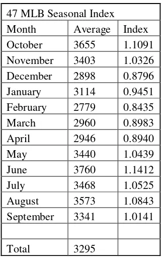
47 MLB Seasonal Index Month Average Index
October 3655 1.1091
November 3403 1.0326 December 2898 0.8796
January 3114 0.9451
February 2779 0.8435
March 2960 0.8983
April 2946 0.8940
May 3440 1.0439
June 3760 1.1412
July 3468 1.0525
August 3573 1.0843
September 3341 1.0141
Total 3295
Table 2: Seasonal Index for 47 MLB
Two Dimension Regressions
A comparison of two regressions that will provide a two-dimension regression formula for operational availability as a function of cost and operating hours as a function of cost, these will show the changes in operational availability and operating hours individually as a function of cost. The expected format for Operating Hours as a function of Cost is a simple linear curve:
R F
The inverse function of H(C) becomes the utility function of C(H):
R R F
The expected form of the function of operational availability as a function of cost is a logarithmic function:
. S F
The inverse function of Ao(C) becomes the single variable or two dimensional utility function of cost or C(Ao):
vw4xy
15
These functions become the single variable form of the utility function for cost. When expected value of the cost is calculated using a single variable the functions of C(Ao) and C(H) are the utility functions.
Statistical Process Control and Normal Distribution
Two major assumptions that will require substantial validation are statistical process control and normal distribution of the variables’ operational availability and operating hours. The process involved does not require more than a 95% certainty that they are accurate, so three standard distributions are acceptable to calculate the upper and lower control limits for each variable. The upper and lower control limits will be calculated about the mean and plotted into a control chart. The control chart will be evaluated on the basis of having the data points with in the upper and lower control limits, trends, and random nature of the plot over time. (Heizer, 2008) As the data sets are not conducive to breaking apart the fleet into specific data samples, the cost data does not assign cost to a specific platform. For example, SBPL does not have the cost of the RB-S carrying the hull number 25401 for each month of the analysis and would be too costly to attempt to figure out for each hull. Thus, the analysis is forced to work with the overall fleet as the sample not individual platforms.
The second assumption is that the operational availability and operating hours are random variables that are normally distributed about the mean. The variables will be plotted into frequency histograms to show the number of times the variable has fallen between specific intervals. Superimposing the normal probability density function for the mean and variance over the histogram will indicate the accuracy of this assumption. (Hogg, 2010) When this assumption is true, the cost will also be a random variable, as the cost is the sum of the products of operational availability.
When these assumptions are true, the cost is also a random variable with a normal distribution, as the function linking the two will involve two random variables being added together. Even though, all of the variables are entirely human controlled, there are so many managers and controllers involved in the process that it forms a normal distribution.
Having two normally distributed random variables will allow the use of the bivariate normal distribution to calculate the pdf of the cost random variable. Cost can also be calculated as a function of x as a traditional two dimensional normal distribution.
Linking Monthly Data to Derive Curve
The data provides a multivariable relationship between cost, operational availability, and operating hours. The cost can then be estimated by calculating the plane as a function of operational availability and operating hours. The plots are then estimated by using the multivariable regression in NCSS. The regression provides a volume when integrated.
", R , R FR A
The general regression provides the relationship between the three variables. This relationship becomes the utility function of the expected value in the three dimension form.
16
cost by keeping the hour fixed at the mean and changing the availability between the upper and lower control limit. The swing squared is then calculated and summed, and a percent variance is calculated.
z!S$ " R!SV " +z$
E!A ∑ z!Sz!S$$
The variable that creates the greatest variance in the cost is the dominant variable, or the controlling variable. (Clemen, 2001)
Expected Value
Calculating the expected value of each model on a monthly basis will show the new lifecycle cost estimate based upon the probability of maintaining the revised operational profiles of the 25 RB-S and the 47 MLB. The end result will be the expected cost of the individual boat classes per month. The expected value does not account for a fleet reduction and assumes a static fleet size. However, dividing by the number of current boats will not give an accurate answer of how much it will cost to operate each boat, because of economies of scale. Because it is cheaper to operate 400 boats of the same kind than 50 of the same kind. The bivariate normal distribution will be used as an estimate of the probability distribution function of the cost variable. It will be called an estimate or approximation due to the use of the sample mean and sample standard deviation. (Hogg, 2010)
Both operating hours and operational availability are continuous variables. The variables have infinite number of points between the limits. Both random variables measure a time period, either by percentage or actual, and by the nature of time being continuous and not discrete. The random variables will be treated as continuous.
The lowest expected value will be the best case in this function. The expected value will be calculated using the bivariate normal distribution and the cost function as a result of operational availability and operating hours. The bivariate normal distribution has defined limits in this case as operational availability is only valid from zero to one for both the 25 RB-S and 47 MLB. The operating hours are also limited as the 47 MLB can only produce between 0 and 84,240 hours and the 25 RB-S can only produce between 0 and 254,400 hours in a 30 day month. Thus the pdf of A and H for the 47MLB is:
1 { /, R M M|},$}~/, R R
~ *
~
And for the 25 RB-S:
1 { /, R M M$},}~~/, RR
~ *
~
17
Models Resulting From a Mandate to Increase Operational Availability
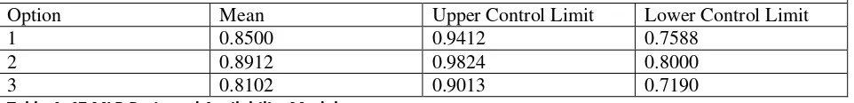
In a cost avoidance effort to reduce acquisition costs related to small boats, the Coast Guard developed and executed what has become known as the Office of Boat Forces Boat Optimization Plan. The plan is based off a linear programing model that accounts for boats as resource hours or operating hours, and focuses heavily on the operations of the Coast Guard with little mention of maintenance time or cost. (Wagner, 2012) The plan was adapted and is in the process of implementation by the Coast Guard. The estimated increase in operational availability is not discussed, but is essential to the full implementation of the plan. This analysis will focus on three options that have been recommended by the Small Boat Product Line. (Keister, Small Boat Product Line Manager, 2013) Option one proposed by CDR Scott Keister is an average boat availability of 0.85, which would result in control limits of three standard deviations above and below. This would be an increase of the target average boat availability for the 25 RB-S and 47 MLB of 0.02 and 0.06, respectively. The second option sets the minimum acceptable operational availability at 0.80 for each boat class, and calculates the mean as three standard deviations above the lower control limit. The third option is to retain the current model and is simply the mean of the previous three years (FY2011-13). Each model maintains the assumption that the operating hours will remain close to the average and within the control limits calculated off of the last three years.
25 RB-S Standard Deviation = 0.0295
25 RB-S Projected Operational Availability Models
Option Mean Upper Control Limit Lower Control Limit
1 0.8500 0.9385 0.7615
2 0.8885 0.9770 0.8000
3 0.8257 0.9142 0.7371
Table 3: 25 RB-S Projected Availability Models
47MLB Standard Deviation = 0.0304
47MLB Projected Operational Availability Models
Option Mean Upper Control Limit Lower Control Limit
1 0.8500 0.9412 0.7588
2 0.8912 0.9824 0.8000
3 0.8102 0.9013 0.7190
Table 4: 47 MLB Projected Availability Models
The analysis will keep the operating hours constant throughout in order to compare the new availability models via expected value or expected cost and lifecycle cost estimates. This will allow the models to be compared without further adjustment.
Lifecycle Cost Estimates
18
By using a programmed spreadsheet to develop random variables within the new controls, projected realistic availabilities were generated. While not forecasts, the assumption was made that the SBPL would maintain the system within the control limits of the model. Thus, a random number could be used as long as it was within the control limits. (Keister, Small Boat Product Line Manager, 2013)
D !F!!N D QF ++ . 1000, + . 1000/10,000
The availabilities are multiplied by 1,000 and divided by 10,000 to maintain the number less than one and so that a new random number program did not have to be programmed. Microsoft Excel random number program uses whole numbers without decimal places.
The hours were generated by assuming the last two years FY12 and FY13 were typical of the rest of the lifecycle of each of the assets. As the current budget posture statement by the Coast Guard Commandant, Admiral Papp indicates the hours will stabilize over the next number of years. (Papp, United States Coast Guard Posture Statement, with 2014 Budget in Brief, 2013) By holding the hours stable for the out years, each model will allow the availability comparisons to be made. The hours model was based upon projections for FY14 and beyond using a random number generator. A second operation is also underway with the 25 RB-S. It is under a recapitalization plan, so the mathematical operation is a ratio that reduces the hours keeping the same level of operating hours. The numbers inserted are based off an assumption made for this analysis that the 25 RB-S will be phased out in the next five years with the last boat being decommissioned on September 30, 2018.
25 DT D RQ"
" C . D QF 1921, 11238 . A QF / T" Q QF / T"
47 +T D RQ" " C . D QF ++, +
This model reflects current normal operations of the Coast Guard and does not reflect a substantial change to the national level operating levels. A significant event such as Hurricane Katrina or major terrorist event could cause a spike in operating hours that could not be foreseen. A different set of requirements with an emergency funding string would potentially need to be enacted. While in the years used to develop the model, Super Storm Sandy struck, it did not cause the massive spike in small boat operations that were seen during Hurricanes Katrina and Rita in September and October of 2005.
19
Chapter 4: 25 RB-S Results
Statistical Process Control
The 25 RB-S operating hours and operational availability were measured each month between October 2009 and September 2013, beginning with Fiscal Year 2010 and ending with Fiscal Year 2013. The base year to calculate control limits was FY10 for both operational availability and operating hours. Three standard deviations were used to determine if the two variables were in control. Operational availability was the first calculated with a sample standard deviation of 0.0295 and a sample mean of 0.8257. The resulting control chart is below, in Figure 2.
Figure 2: 25 RB-S Operational Availability Control Chart
The 25 RB-S falls randomly within the upper and lower control limits with normal variation. When the data is plotted in a histogram, it appears to have a normal distribution about the mean, Figure 2. The result is the 25 RB-S system or fleet and both mechanically and logistically is within statistical process control in regards to operational availability. The probability mass function is plotted as well, in the generic format of:
/ 1
3√22
4 647$89 9
0.5 0.55 0.6 0.65 0.7 0.75 0.8 0.85 0.9 0.95 O ct -0 9 Ja n -1 0 Ap r-1 0 Ju l-1 0 O ct -1 0 Ja n -1 1 Ap r-1 1 Ju l-1 1 O ct -1 1 Ja n -1 2 Ap r-1 2 Ju l-1 2 O ct -1 2 Ja n -1 3 Ap r-1 3 Ju l-1 3 O p e rat io n al A v ai lab il it y
25 RB-S Operational Availability Control Chart
Operational Availability
Upper Control Limit
Lower Control Limit
20 Figure 3: 25 RB-S Operational Availability Histogram
0 5 10 15
25 RBS Operational Availability
Histogram
21
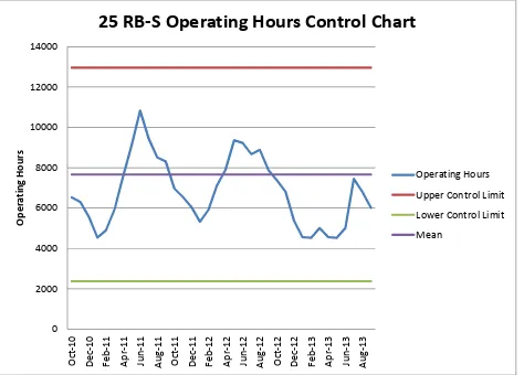
Operating hours were also placed into control charts and histograms. The 25 RB-S operating hours has a sample standard deviation of 1,763 Hours and a sample mean of 7,665 Hours, Figure 3 depicts the operating hours control chart. The operating hours as previously discussed are seasonal due to the lower levels of operations from late fall to early spring.
Figure 4: 25 RB-S Operating Hours Control Chart
The operating hours fall into the control limits and take a fairly random nature in the controls after considering the seasonal nature of the operating hours. Also of interest is the reduction in operating hours in FY13 and where operating hours no longer follow their natural seasonality. This is most likely due to the impacts of the Budget Control Act of 2011 that placed a cap and reduced government spending. Reducing operating hours is seen as a simple and easy-to-implement strategy to reduce budget costs. Thus, there is a cost savings, as fuel is not consumed and equipment does not face the wear and tear as it would while underway. (Papp, ALCOAST 074/13 Subj: Shipmates 24 - Potential Sequestration, 2013) The operating hours follows a normal distribution as well, except for it being truncated at the lower end, Figure 4. Again, the normal distribution is plotted on the histogram with the points being the average of the division upper and lower limit.
0 2000 4000 6000 8000 10000 12000 14000 O ct -1 0 D e c-1 0 F e b -1 1 Ap r-1 1 Ju n -1 1 Au g -1 1 O ct -1 1 D e c-1 1 F e b -1 2 Ap r-1 2 Ju n -1 2 Au g -1 2 O ct -1 2 D e c-1 2 F e b -1 3 Ap r-1 3 Ju n -1 3 Au g -1 3 O p e rat in g H o u rs
25 RB-S Operating Hours Control Chart
Operating Hours
Upper Control Limit
Lower Control Limit
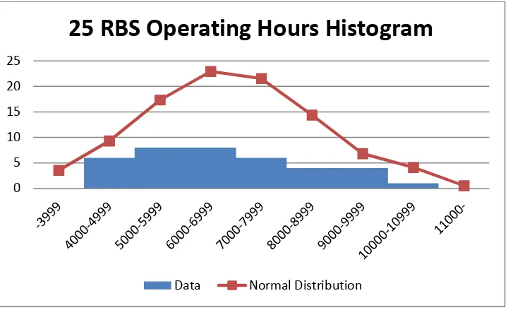
22 Figure 5: 25 RB-S Operating Hours Histogram
The histogram is truncated and no month has fallen below 4,000 hours. This is due to a minimum training requirement for all coxswains and boat crew to maintain proficiency at operating the boats. Each coxswain and crew member must have 36 hours total with 10%, or 3.6, of those hours being at night every six months. This minimum for crew proficiency skews the operating hours higher than what there would be if there were no minimum hours for proficiency. There is no perceived cost savings by eliminating the underway hour’s proficiency requirement as there are higher potential for accidents and loss or damage due to them. (Cross, 2002) The end result is that the operating hours are as randomly distributed as the actual data will allow and do fall within the control limits, even with the reduced operating hours in FY13.
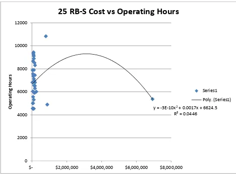
Cost Versus Operating Hours
The cost versus operating hours was plotted in an x-y scatter, and a regression was performed to validate the measure of maintenance cost per operating hour. This is a current measure used by the Coast Guard Headquarters Staff, SFLC, and SBPL to measure performance of the product line. On average in FY12 (the latest year available), the 25 RB-S cost $38 per operating hour. The number fluctuates with operating hours and dollars spent over the year. The regression will show the relationship between the dollars spent and the operating hours by showing the operating hours as a function of cost, Figure 6.
0 5 10 15 20 25
25 RBS Operating Hours Histogram
23 Figure 6: 25 RB-S Cost versus Operating Hours
The regression was done as a polynomial as the model provided the best relationship of the various regression models attempted. The original thought was that the regression would be linear, as one would expect the more you pay, the more operating hours one would get. Skewing the data is the data point from December 2012, when SBPL spent nearly $7 million on the 25 RB-S system when the system had relatively low hours in that month. This expense was necessary, as the positive effects are seen through the remainder of the fiscal year in increased operational availability.
y = -3E-10x2+ 0.0017x + 6624.5
R² = 0.0446
0 2000 4000 6000 8000 10000 12000
$- $2,000,000 $4,000,000 $6,000,000 $8,000,000
O
p
e
rat
in
g
H
o
u
rs
25 RB-S Cost vs Operating Hours
Series1
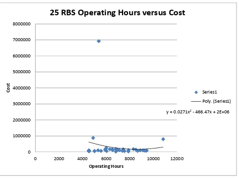
24 Figure 7: 25 RB-S Operating Hours versus Cost
A second regression was run having cost as a function of operating hours which results in the separate linear polynomial expression. The resulting function:
R 0.0271R$ 466.47R 2,000,000
Cost versus Operational Availability
Similarly to the cost versus operating hours, the same plot and regression were run with cost and operational availability to determine the type of relationship. The plot with trend line is predicted by the OPNAV INST, stating that the expected curve is a logarithmic curve, thus the regression was performed with the use of the logarithm model, Figure 8.
y = 0.0271x2- 466.47x + 2E+06
0 1000000 2000000 3000000 4000000 5000000 6000000 7000000 8000000
0 2000 4000 6000 8000 10000 12000
C
o
st
Operating Hours
25 RBS Operating Hours versus Cost
Series1
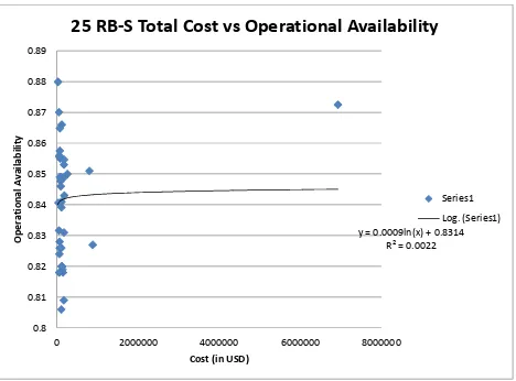
25 Figure 8: 25 RB-S Total Cost vs Operational Availability
The expected curve per the OPNAV has a limit of 1 as the dollars, or cost, goes toward infinity; this is true for this regression. (Moore, 2003) Although the regression nearly has no slope, the more data added, the stronger the relationship will become, and the more positive the slope, as data with greater variation is collected.
vw)*)Olim 0.0009 . ln 0.8314
With,
Ao = Operational Availability
C = Cost
Manipulating the regression to have cost as a function of availability results in:
vw4~.|*}~.~~~$
Which respects the limit of Ao still being 1, as cost is infinite.
y = 0.0009ln(x) + 0.8314 R² = 0.0022
0.8 0.81 0.82 0.83 0.84 0.85 0.86 0.87 0.88 0.89
0 2000000 4000000 6000000 8000000
O
p
e
rat
io
n
al
A
v
ai
lab
il
it
y
Cost (in USD)
25 RB-S Total Cost vs Operational Availability
Series1
26
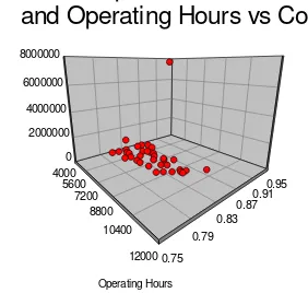
Multi-Regression of Cost as a function of Operational Availability and Operating Hours
A multi-regression was run in NCSS to determine the interrelationship between cost, operational availability and operating hours. (Hintze, 2004) This regression resulted in a linear formula that estimated the function of the three-dimensional plot, Appendix A.
Figure 9: 3-D Plot of Cost as a function of Operational Availability and Operating Hours
The resulting regression formula from this regression is:
, R 22781100 . 17.10694 . R 18660110
With
"
W! !F!!N R W!S RQ"
The regression formula was run through a sensitivity analysis to determine if a controlling or dominate variable exists. The upper and lower control limits were used to calculate the high and the low with the mean as the control.
25 RBS Operational Availability
and Operating Hours vs Cost
C
o
s
t
(U
S
D
)
Operational Availability
Operating Hours
0.75 0.79
0.83 0.87
0.910.95 0
2000000 4000000 6000000 8000000
4000 5600
7200 8800
27 Table 5: 25 RB-S Sensitivity Analysis
Operational availability is dominating in the cost equation and accounts for 0.9980 of the change in cost. One could also say for every dollar spent on the 25RB-S system $0.99 goes toward paying for operational availability. The cost equation is based on normal operations and maintenance of the 25 RB-S and does not include any costs of a mid-life or recapitalization effort. The fact that operational availability so heavily controls the cost equation intuitively makes sense as the mission of the 25 RB-S is to respond to emergencies more than complete scheduled patrols. The mindset of the operational commander, or customer, is more that of “how many boats do I have ready to go today” than how many hours have my boats completed. This is important when creating this metric and measuring the amount of operational availability, as this is also the loan variable that the mission support organization of the Coast Guard controls and is out of the hands of the operational commander.
Bivariate Normal Distribution
The bivariate normal distribution was plotted for the 25 RB-S between the upper and lower control limits of the operational availability and the operating hours. Similarly to the normal distribution in the two-dimension form when integrated using both variables is equal to the probability.
Figure 10: 25 RB-S Bivariate Normal Distribution Graph
Variable Low Mean High Low Cost Base Cost High Cost Swing Swing^2 % Var
Hours 2375 7665 12955 109615.2875 19119.57 -71376.1 -180991.43 32757895996 0.002008428
Availability 0.7371 0.8257 0.9142 -1999285.89 19119.57 2035247 4034532.8 1.62775E+13 0.997991572
1.63102E+13
25 RBS Bivariate Normal
Distribution Graph
J
o
in
t
P
ro
b
a
b
ili
ty
Operating Hours Operational Availability
0.7
0.9 0.00000
0.00600
2000.0
28
Figure 10, is a graphical representation of the 25 RB-S pdf using the bivariate normal distribution. (Hintze, 2004)
Expected Cost
Calculating the expected value or expected cost of the 25 RB-S using the multivariable cost function and the bivariate normal probability distribution function. The multivariable cost regression becomes the utility function and the bivariate normal probability distribution function is the pdf. Because the variables of operational availability and operating hours are interrelated it would make senses that the correlation coefficient (ρ) is not equal to zero, this is true for the 25 RB-S. The concept being that in order for the boat to get underway and produce operational hours it must be operationally available. The resulting equations:
, R 22781100 . 17.10694 . R 18660110
/, R 1
223vw3#1 @$ 4 *
$#*4K9Gvw478I 9
4$KGvw47
8 IG478IJG478I 9
3vw 0.018662
vw 0.841501
3 1709.563
6817.563
@ 0.141609
P> M M , R . /, RR
**,$|
*,$* v
v
Option Amin Amax E[X]
1 0.7615 0.9385 $3,427,420
2 0.800 0.977 $3,582,660
3 0.7371 0.9142 $3,331,110
Table 6: 25 RB-S Operational Availability Models
29
Lifecycle Cost Estimate
The total lifecycle cost for each option available was calculated using a normally distributed random number generator with in each new operational availability distribution. The operating hours account for the seasonality of the operating hours variable, and the total cost is reduced through the remainder of the lifecycle by a factor based on the reduction of fleet size from month to month based upon deliveries of 29 RB-S Generation II and the boat optimization plan. The results are presented in Table 7
Option Estimated Total Lifecycle Cost
1 $33,431,847
2 $44,685,253
3 $33,529,491
Table 7: 25 RB-S Estimated Total Lifecycle Cost
30
Chapter 5: 47 MLB Results
Statistical Process Control
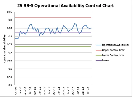
The 47 MLB operating hours and operational availability were measured each month from October 2009 to September 2013, all months in FY11 thorough FY13 inclusive. The base year was FY10 to calculate statistical limits. The first calculated control limits were for operational availability, which had a mean of 0.8102 and a standard deviation of 0.0304. The three years were then plotted with the control limits set at three standard deviations from the mean; the resulting control chart is in Figure 10.
Figure 11: 47 MLB Operational Availability Control Chart
There are several reasons for the 47 MLB being out of statistical control, the first is system age and obsolescence. The 47 MLB was designed and constructed prior to Environmental Protection Agencies (EPA) Tier II requirements were in place. Although the boat is grandfathered for continued operations, the main propulsion engine is no longer manufactured on a large scale. Meaning that as the engine fleet ages, it requires increasingly scarce parts that are expensive and take time to manufacture, thus increasing delays in supply and logistics. The downward trend over the twelve-month period from May 2012 to April 2013 is indicative of the problems within the 47 MLB as a whole system. The fact that FY2013 never saw an operational availability above the mean from FY2010 shows that the system has accepted a lower level of operational availability. This is indicative of the out of control roller coaster effect in that the process will continue to produce; however, significant upward and downward trends will continue to be the norm unless the system is changed in some manner.
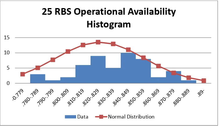
The Operational Availability was also plotted into a histogram to assess the distribution of the random variable. The resulting distribution was approximated using a normal distribution curve, in figure 11.
0.5 0.55 0.6 0.65 0.7 0.75 0.8 0.85 0.9 0.95 1 O ct -1 0 D e c-1 0 F e b -1 1 Ap r-1 1 Ju n -1 1 Au g -1 1 O ct -1 1 D e c-1 1 F e b -1 2 Ap r-1 2 Ju n -1 2 Au g -1 2 O ct -1 2 D e c-1 2 F e b -1 3 Ap r-1 3 Ju n -1 3 Au g -1 3 O p e rat io n al A v ai lab il it y
47 MLB Operational Availability Control Chart
Operational Availability
Upper Control Limit
Mean
31 Figure 12: 47 MLB Operational Availability Histogram
The three-year period has a relatively normal distribution; however, the problem becomes the defined trends that were discussed with the control chart. The normal distribution does provide a good estimate of the distribution of operational availability for the operational availability and that it is a random variable.
The Operating Hours of the 47 MLB were also plotted into a statistical control chart, again with the control year being FY2010. The mean was 3,725 hours with a standard deviation of 310 hours; the resulting control chart is in figure 12.
0 2 4 6 8 10 12 14
Operational Availability
32 Figure 13: 47 MLB Operating Hours Control Chart
The operating hours are out of statistical control for the 47 MLB, discounting the seasonality of the variable the hours consistently dropped below the lower control limit each year in early spring. In FY2013 this drop below was extended into March and April most likely as a result of the Budget Control Act. Each year is consistent with the overall downward trend in operating hours, however FY2013 does not reach the mean level of FY2010, this indicates a shift in the mean over the time period, and most likely a change in the way the operational commanders are using the 47 MLB.
A histogram plot of the monthly operating hours shows relatively normal distributions with the 36 months are looked at as the sample.
2000 2500 3000 3500 4000 4500 5000 O ct -1 0 D e c-1 0 F e b -1 1 Ap r-1 1 Ju n -1 1 Au g -1 1 O ct -1 1 D e c-1 1 F e b -1 2 Ap r-1 2 Ju n -1 2 Au g -1 2 O ct -1 2 D e c-1 2 F e b -1 3 Ap r-1 3 Ju n -1 3 Au g -1 3 O p e rat in g H o u rs
47 MLB Operating Hours Control Chart
Operating Hours
Upper Control Limit
Mean
33 Figure 14: 47 MLB Operating Hours Histogram
In figure 13, the red line shows the calculated normal distribution for the operating hours. The distribution appears to be, for the most part, random although the data is denser in the lower operating hour’s levels. It can be concluded that the operating hours of the 47 MLB are random around the mean with the exception of the seasonality inherit in the data for operating hours.
Cost Versus Operating Hours
The operating hours as a function of the cost were plotted and a regression run for the 47 MLB, shown in figure 14.
0 1 2 3 4 5 6 7 8 9
Operational Availability
34 Figure 15: 47 MLB Cost versus Operating Hours
The resulting regression shows a decreasing number of operating hours as more funding is invested. Two potential causes are in play, first are planned depot maintenance (PDM) costs from dry dock availabilities to prevent the boats from performing underway hours. Some significant delays have potential to not only increase cost but also reduce operating hours. The second factor that is in play is the increased cost of material and across the board reduction in operating hours. Both factors contribute to the deficit however neither is entirely responsible.
Cost versus Operational Availability
Similarly to operating hours, operational availability was plotted as a function of cost, the resulting graph and regression is below in figure 15.
y = -0.0001x + 3346.1 R² = 0.0022
2000 2500 3000 3500 4000 4500
0 200000 400000 600000 800000 1000000 1200000
O
p
e
rat
in
g
H
o
u
rs
Cost
47 MLB Cost vs Operating Hours (FY11-FY13)
Series1
35 Figure 16: 47 MLB Cost versus Operational Availability
The resulting curve has a negative slope, which is not the predicted slope. The negative slope is due to the increasing costs of maintaining an obsolete system, as described in the latest Ships Structure and Machinery Evaluation Board. (Keffer, 2010) The resulting formula does not mean that the less funding the SBPL expends the higher the operational availability, in actuality the inverse is true. Cost is increasing and less operational availability is being produced for many of the same reasons of the trending nature of the operational availability variable.
Multi-Regression of Cost as a Function of Operational Availability and Operating Hours
The cost regression as a function of operational availability and operating hours was run in NCSS. (Hintze, 2004) The resulting plot and regression is in Figure 16.
y = -0.015ln(x) + 0.9806 R² = 0.0232
0.5 0.55 0.6 0.65 0.7 0.75 0.8 0.85 0.9 0.95 1
0 200000 400000 600000 800000 1000000 1200000
O
p
e
rat
io
n
al
A
v
ai
lab
il
it
y
Cost
47 MLB Cost vs Operational Availability
Series1