University of New Orleans University of New Orleans
ScholarWorks@UNO
ScholarWorks@UNO
University of New Orleans Theses and
Dissertations Dissertations and Theses
5-20-2005
A Multi-Dimensional Width-Bounded Geometric Separator and its
A Multi-Dimensional Width-Bounded Geometric Separator and its
Applications to Protein Folding
Applications to Protein Folding
Sorinel Oprisan
University of New Orleans
Follow this and additional works at: https://scholarworks.uno.edu/td
Recommended Citation Recommended Citation
Oprisan, Sorinel, "A Multi-Dimensional Width-Bounded Geometric Separator and its Applications to Protein Folding" (2005). University of New Orleans Theses and Dissertations. 238.
https://scholarworks.uno.edu/td/238
A MULTI-DIMENSIONAL WIDTH-BOUNDED GEOMETRIC SEPARATOR AND ITS APPLICATIONS TO PROTEIN FOLDING
A Thesis
Submitted to the Graduate Faculty of the University of New Orleans
in partial fulfillment of the requirements for the degree of
Master of Science in
Computer Science
by
Sorinel Adrian Oprisan
B.S. “Alexandru Ioan Cuza” University of Iasi, Romania, 1987 Ph.D. “Alexandru Ioan Cuza” University of Iasi, Romania, 1998
Dedication
Acknowledgments
I would like to give my sincere thanks to Dr. Bin Fu for his guidance, patience and supervision during my graduate work.
Contents
Abstract v
1 Introduction 1
1.1 Proteins and amino acids . . . 1
1.2 Proteins structure . . . 3
1.3 Protein folding . . . 6
1.4 HP model of protein folding . . . 8
2 Multi-Directional Width-Bounded Geometric Separator 13 2.1 Overview of our method . . . 14
2.2 Separators upper bound for grid graphs . . . 15
2.3 Separator lower bound for grid graphs . . . 19
2.4 Shortest separator of the unit circle . . . 23
3 Application of multi-directional width-bounded geometric separators to protein folding in the HP model 27 4 Upper bounds for multi-directional width-bounded geometric separators in rectangular and triangular lattices 35 4.1 Two-dimensional rectangular lattice . . . 35
4.2 Two-dimensional triangular lattice . . . 41
5 Conclusions 49
Bibliography 54
Abstract
We used a divide-and-conquer algorithm to recursively solve the two-dimensional problem of protein folding of an HP sequence with the maximum number of H-H contacts. We derived both lower and upper bounds for the algorithmic complexity by using the newly introduced concept of multi-directional width-bounded geometric separator. We proved that for a grid graph G with n grid points P, there exists a balanced separator A ⊆ P such that A has less than or equal to 1.02074√n points, and G-A has two disconnected subgraphs with less than or equal to 2
3n nodes on each subgraph. We also derive a 0.7555
√
n lower bound for our balanced separator. Based on our multi-directional width-bounded geometric separator, we found that there is an O(n5.563√n) time algorithm for the 2D protein folding problem
Chapter 1
Introduction
In the year 2000, a distinguished panel of renowned scientists at the U.S. National Research Council identified six fundamental challenges to the scientific community [1]: (1) Developing quantum technologies, (2) Understanding complex systems, (3) Applying physics to biology, (4) Creating new materials, (5) Exploring the Universe, and (6) Unifying the forces of Nature. For computational biology, “Current challenges include [...] the (study of) mechanical and electrical properties of DNA and the enzymes essential for cell division and all cellular processes.”
The behavior of complex systems, such as the proteins, depends crucially on the molecular details and therefore it seems unlikely that the traditional reductionist way would succeed in this field. For example, small perturbations of a protein’s environment such as alterations of the pH or substitutions of just one amino acid in the chain might change dramatically the folding process and the biological activity of the protein. The allosteric proteins which drastically alter their shape and properties when they link a small regulating molecule (like a vitamin) are a good example of sensitivity of the global structure to small molecular details.
1.1
Proteins and amino acids
Protein etymology comes from the Greek word “proteios”, which means first. Next to water, proteins make up the second greatest portion of a person’s body weight.
the essential role to catalyze, regulate, and protect the cell’s chemistry. For example, the hemoglobin, myoglobin and various lipoproteins are responsible for the transport of oxygen and other substances within an organism. Proteins are generally regarded as beneficial, and are a necessary part of the diet of all animals. However, some proteins such as the venoms of many snakes, and ricin (extracted from castor beans), are extremely toxic. A teaspoon of botulinum toxin A, from Clostridium botulinum, would be sufficient to kill a fifth of the world’s population. The toxins produced by tetanus and diphtheria microorganisms are nearly as poisonous. Allergies are generally caused by the effect of foreign proteins on our body. Proteins that are ingested are broken down into smaller peptides and amino acids by digestive enzymes called “proteases”. Allergies to foods may be caused by the inability of the body to digest specific proteins. Cooking denatures (inactivates) dietary proteins and facilitates their digestion. Allergies or poisoning may also be caused by exposure to pro-teins that bypass the digestive system by inhalation, absorption through mucous tissues, or injection by bites or stings.
From a chemical point of view, proteins’ composition is significantly different compared to the carbohydrates and lipids. Lipids are largely hydrocarbon in nature, generally being 75-85% carbon. Carbohydrates are roughly 50% oxygen, and like lipids, usually have less than 5% nitrogen (often none at all). Proteins, on the other hand, are composed of 15-25% nitrogen and about an equal amount of oxygen.
Proteins consist of amino acids which are characterized by the -CH(NH2)COOH substruc-ture (Figure 1.1A). Nitrogen and two hydrogen atoms comprise the amino group, −NH2,
and the acid entity is the carboxyl group, −COOH. Amino acids are the basic building blocks of enzymes, hormones, proteins, and body tissues. A peptide is a compound consist-ing of 2 or more amino acids. Oligopeptides have 10 or fewer amino acids. Polypeptides and proteins are chains of 10 or more amino acids, but peptides consisting of more than 50 amino acids are classified as proteins.
Amino acids link to each other when the carboxyl group of one molecule reacts with the amino group of another molecule, creating a peptide bond −C(=O)NH− and releasing a molecule of water (Figure 1.1B).
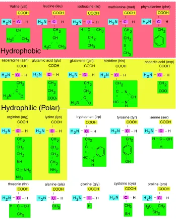
There are twenty different amino acids characterized by variations in their side chain (Figure 1.2). Some amino acids are called essential because they cannot be derived from other amino acids and must be supplied in the diet (isoleucine, histidine, leucine, lysine, methionine, threonine, tryptophan, valine).
C H N2 _ _
_ _ H COOH R α C _ _ R H _ _
H N2 _ C
_ _ _ H _ H _
H __ C H _ R _ C _ _ _ _ H A B C _ _ R H _ _
H N2 _ C
_ H _ C _ H _ R _ C _ _ _ _ H _ _
+ H O2
Figure 1.1: (A) Planar structure of amino acids contains an amino group (−NH2), the
carboxyl group (-COOH) and the α carbon. (B) Peptide bond created by interaction of amino group of one molecule with the carboxyl groups of another molecule after releasing one molecule of water.
therefore, reside predominantly in the interior of proteins. This class of amino acids does not ionize nor participate in the formation of H-bonds. The hydrophilic amino acids tend to interact with the aqueous environment, are often involved in the formation of H-bonds and are predominantly found on the exterior surfaces proteins or in the reactive centers of enzymes.
Among the well-known peptide hormones, we mention vasopressin, which contains 9 amino acids and increases the reabsorption rate of water in kidneys; insulin, which contains 51 amino acids and is involved in lowering the blood glucose level; growth hormone, which contains 191 amino acids and regulates development of the body [15, 42, 55].
1.2
Proteins structure
Proteins have multiple structural levels. The most basic structure of proteins is called the
primary structure, which is simply the order of its amino acids. Note that by convention, the order of amino acids in a protein is always written from the amino group end to the carboxyl group end.
Secondary Structure
C H N2 _ _
_ _ H COOH CH _ _
H C3 CH3 Valine (val)
C H N2 _ _
_ _ H COOH CH _ _
H C3 CH3 CH2
_
leucine (leu)
C H N2 _ _
_ _ H COOH CH2 _ C H _ _ CH3
_
CH3 isoleucine (ile)
C H N2 _ _
_ _ H COOH CH2 _ CH3 CH 2 S _ _ methionine (met) C H N2 _ _
_ _ H COOH CH2 _ phynialanine (phe) _ C C H N2 _ _
_ _ H COOH _ _ CH2 _
H N2 O asparagine (asn)
C H N2 _ _
_ _ H COOH CH2 _ CH2 COO-_
glutamic acid (glu)
C H N2 _ _
_ _ H COOH CH2 _ CH2 _ _ C _ _
H N2 O glutamine (gln) CH _ H C C H N2 _ _
_ _ H COOH CH 2 _ _ _ _ HC _N
_ N
_
histidine (his)
C H N2 _ _
_ _ H COOH CH 2 _ CH 2 _ CH 2 _ CH 2 _ NH2 lysine (lys) _ __ C C H N2 _ _
_ _ H COOH CH 2 _ CH2 _ CH2 _ NH 2 _ NH NH2 arginine (arg) C H N2 _ _
_ _ H COOH CH 2 _ COO aspartic acid (asp)
C H N2 _ _
_ _ H COOH H glycine (gly) C H N2 _ _
_ _ H COOH CH3 alanine (ala) C H N2 _ _
_
_
H COOH
C _ OH _ H _ H serine (ser) C H N2 _ _
_
_
H COOH
C _ OH _ H _ CH3 threonin (thr) C H N2 _ _
_ _ H COOH CH _ 2 _ OH tyrosine (tyr) C H N2 _ _
_ _ H COOH CH _ 2 _ C _ HC _ _ N H _ tryptophan (trp) C H N2 _ _
_ _ H COOH CH _ 2 SH cysteine (cys) C H N2 _ _
_
_
H COOH
CH
_ _ 2
CH 2 H C
_
2 proline (pro)
Hydrophobic
Hydrophilic (Polar)
Figure 1.2: Structural formulas for the twenty natural amino acids.
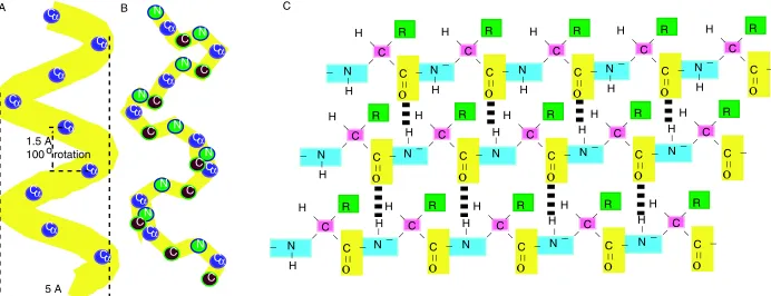
makes up the central structure, and the side chains extend out and away from the helix. The carboxyl group of one amino acid (n) is hydrogen bonded to the amino group of the amino acid four residues away (n+4). Alpha-helix structure was first postulated by Linus Pauling (Nobel Prize for chemistry in 1954), Robert Corey, and Herman Branson in 1951 based on the known crystal structures of amino acids and peptides and Pauling’s prediction of planar peptide bonds [24].
1 A A S X D X S L V E V H X X V F I V P P X I L Q A V V S I A
31 T T R X D D X D S A A A S I P M V P G W V L K Q V X G S Q A
61 G S F L A I V M G G G D L E V I L I X L A G Y Q E S S I X A
91 S R S L A A S M X T T A I P S D L W G N X A X S N A A F S S
121 X E F S S X A G S V P L G F T F X E A G A K E X V I K G Q I 151 T X Q A X A F S L A X L X K L I S A M X N A X F P A G D X X 181 X X V A D I X D S H G I L X X V N Y T D A X I K M G I I F G 211 S G V N A A Y W C D S T X I A D A A D A G X X G G A G X M X 241 V C C X Q D S F R K A F P S L P Q I X Y X X T L N X X S P X 271 A X K T F E K N S X A K N X G Q S L R D V L M X Y K X X G Q 301 X H X X X A X D F X A A N V E N S S Y P A K I Q K L P H F D 331 L R X X X D L F X G D Q G I A X K T X M K X V V R R X L F L 361 I A A Y A F R L V V C X I X A I C Q K K G Y S S G H I A A X 391 G S X R D Y S G F S X N S A T X N X N I Y G W P Q S A X X S 421 K P I X I T P A I D G E G A A X X V I X S I A S S Q X X X A 451 X X S A X X A
Table 1.1: The primary structure of the sequence of yeast hexokinase from the yeast species Saccharomyces cerevisiae (http://www.pdb.bnl.gov/pdb-bin/pdbmain). The letters repre-sent abbreviated notations for the corresponding amino acids (see Figure 1.2).
5 A 1.5 A 100 rotationo
Cα Cα Cα Cα Cα Cα Cα Cα Cα Cα Cα Cα Cα Cα Cα Cα Cα Cα N N N N N N N N N C C C C C C C C C A B H C _ _ R H _ _ N _ C
_ _ _ _ _ H C _ _ R H _ _ N _ C
_ _ _ _ H C _ _ R H _ _ N _ C
_ _ _ _ H C _ _ R H _ _ N _ C
_ _ _ _ H C _ _ R H _ _ N _ C
_ _ _ H C _ _ R H _ _ N _ C
_
_
_
_ _
H _C
_
R H _
_ N _ C
_
_
_ _
H _C
_
R H _
_ N _ C
_
_
_ _
H _C
_
R H _
_ N _ C
_
_
_ _ H _C
_
R H _
_ N _ C
_ _ _ H C _ _ R H _ _ N _ C
_
_
_
_ _
H _C
_
R H _
_ N _ C
_
_
_ _
H _C
_
R H _
_ N _ C
_
_
_ _
H _C
_
R H _
_ N _ C
_
_
_ _ H _C
_
R H _
_ N _ C
_
_
_ C
Figure 1.3: Secondary structures of proteins. (A) Alpha-helix backbone formed byαcarbons and (B) a more detailed view of alpha-helix secondary structure including nitrogen atom of the amino group and carbon atom of the carboxyl group. (C) Beta-pleated sheet secondary characterized by hydrogen bonds between hydrogen atoms of amino group and the oxygen atom of carboxyl group with a periodicity of three atoms.
Tertiary Structure
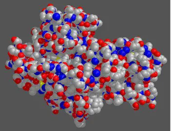
Tertiary structure is the full 3-dimensional folded structure of the polypeptide chain (Figure 1.4).
Quaternary Structure
Quaternary structure is only present if there is more than one polypeptide chain and represents the interconnections and organization of the peptides.
Figure 1.4: Tertiary structure of hexokinase.
1.3
Protein folding
The study of protein synthesis was for many years marked by the so-called “blind watch-maker paradox” [18] and it equates the vastness of the sequence space of polypeptides with the impossibility of ever finding a protein-like sequence. For example, a protein containing only 100 natural amino acids has 20100 ≈ 10130 possible sequences. Therefore, the
the “paradox” is that the probability to obtain an amino acid sequence that folds to the desired 3D shape is much higher than 10−130due to an enormous degeneracy of the sequence
space. It turns out that the probability to obtain a certain 3D conformation is of the order of 10−10 [13,20], which is still small but is reasonable to assume that it could have happened
by natural selection. Moreover, exact models [7] show that the precise information of the sequence is, most of the times, redundant. It has been found that the fold is primarily de-termined by the sequence written in a two-letter alphabet (hydrophobic (H) and polar (P)) rather than in the natural twenty-letter alphabet. Using this code, it was found that, if a certain sequence does fold, the sequence obtained by interchanging one hydrophobic amino acid for another hydrophobic amino acid (similarly for polar ones) will fold with a very high probability to a very similar structure. Thus, the essential features of the full 20100 ≈10130
sequences space remain in the smaller space of the sequences written in the HP alphabet, which contains only 2100 ≈1030 elements.
The second “paradox” of protein folding regards the folding time and is known as the Levinthal paradox [34]. If the protein scans the whole configuration space during folding then the protein will never fold to its native structure. For example, even for a small protein containing only 100 amino acids it can take up to 10 different conformations on average. This makes a total of 10100 different conformations for the chain. If the conformations were
sampled in the shortest possible time, which is about 10−13s, one would need more then 1077
years to sample all the conformational space. This result implies that the protein folding cannot be a completely random trial-and-error process and we must explain how the system can scan such a huge conformation space in going from the unfolded state to the native conformation in such a short time.
The goal of protein folding study is to determine how proteins so consistently fold into a stable state and to understand the complete dynamics and/or chemical changes involved in going from an unfolded linear state into a compact folded state. Although naturally posed as a numerical simulation, there are several problems of scale, including the small energy differences between folded and unfolded states, and the extremely short interval (approximately 10−15 seconds) for which the dynamics equations remain valid, compared
1.4
HP model of protein folding
A protein can fold into a specific 3D structure, which is uniquely determined by the sequence of amino acids. One of the most important problems in molecular biology is determining a protein’s 3D structure from its amino acid sequence. A protein’s 3D structure determines its function. The standard procedure to determine a 3D structure is to purify the protein and crystallize it, followed by x-ray crystallography. It is a very time consuming process and not every protein can be crystallized. Therefore, protein structure prediction with computational technology is one of the most significant problems in bioinformatics.
One of the most popular models of protein folding is the hydrophobic-hydrophilic (HP) model [13, 19, 31]. In the HP model, only two types of monomers are distinguished: hy-drophobic (H), which tend to bundle together to avoid surrounding water, and polar or hydrophilic (P), which are attracted to water and are frequently found on the surface of a folding [13]. These monomers are strung together in some combination to form an HP chain, either an open chain (path or arc) or a closed chain (cycle or polygon).
Usually, the proteins are folded onto the regular square lattice. More formally, a lattice embedding of a graph is a placement of vertices on distinct points of the (regular square) lattice such that each edge of the graph maps to two adjacent (unit-distance) points on the lattice. The space in which the protein folds is discretized by defining a lattice and requiring residues to lie only on lattice points. Residues which are adjacent in the primary sequence (i.e. covalently linked) must be placed at adjacent points in the lattice. A fold of a protein is a self-avoiding walk along the lattice. A contact between two residues is a topological contact if they are not covalently linked and there is an edge connecting the lattice points of the two residues. The free energy of a folded protein in the HP model is defined to be (−1)× the number of topological contacts between pairs of hydrophobic residues. The target fold for the protein is the one which has the lowest free energy. Intuitively, if a protein is folded to bring together many hydrophobic monomers (H nodes), then those monomers are hidden from the surrounding water as much as possible (Figure 1.5). An optimal embedding is one that maximizes the number of H-H contacts. This combinatorial model is attractive in its simplicity, and captures essential features of protein folding such as the tendency for the hydrophobic components to fold to the center of a globular (compactly folded) protein [13]. Unlike more sophisticated models of protein folding, the main goal of the HP model is to explore broad qualitative questions about protein folding such as whether the dominant interactions are local or global with respect to the chain [20].
y
sequence: HPPHPPHPHPPHPPPHHH
A B
y
H
P
H P
-1
0 0
0
E = -4 E = -8
A B
x x
1
1
Figure 1.5: Folding of an HP sequence in a rectangular lattice. An H monomer is represented by a filled circle and a P monomer by an open circle. The free energy of an H-H topological contact (not covalently linked H monomers) is -1 and for any other topological contacts is zero. The free energy of the configuration (A) can be increased by a tighter packing of the hydrophobic core (B).
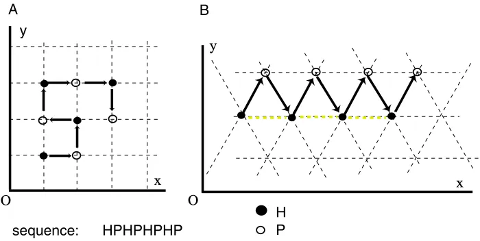
of the relative simplicity of the configuration space. However, square lattice configurations suffer from the so-called “parity problem” in which two residues of even distance from each other in the primary sequence cannot be placed in contact with each other regardless of how one arranges the intervening sequence (Figure 1.6). This parity restriction is clearly an artificial limitation introduced by the specific symmetry of the embedding and is not present when considering the real folding of proteins. For this reason, we also consider protein folding in the HP model on triangular lattices which does not exhibit the parity problem (Figure 1.6). We also note that the free energy of a configuration strongly depends on the symmetry of the embedding.
In theoretical computer science, Berger and Leighton [8, 11] proved NP-completeness of finding the optimal folding in 3D, and Crescenzi et al. [17] proved NP-completeness in 2D.
y
sequence: HPHPHPHP
H P
A B
Figure 1.6: (A) Folding of an HP sequence in a rectangular lattice. For the particular case of (HP)n sequence there is no topological contact between H monomers. (B) Folding of the
same HP sequence in a triangular lattice leads to a significantly lower free energy of the configuration.
Another approach is to develop polynomial time approximation algorithms for the pro-tein folding in the HP model [2–4, 30, 41]. Hart and Istrail [30] have developed a 3/8-approximation in 3D and a 1/4- 3/8-approximation in 2D of the number of H-H contacts in the HP model. Agarwala et al. [3] developed constant-factor approximation algorithms for a generalized HP model allowing multiple levels of hydrophobicity in the 2D triangular lat-tice and the 3D face-centered cube latlat-tice. Newman [41] derived a polynomial time 1/3 -approximation algorithm for the 2D problem.
If the first letter of a HP sequence is fixed at a position of 2D (3D) plane (space), we have at least 2n−1 (3n−1) ways and at most 3n−1 (5n−1) ways to put the rest of the letters on the
plane (space). As the average number of amino acids of proteins is between 400 to 600, if an algorithm could solve the protein structure prediction with about 1000 amino acids, it would be able to satisfy most of the application demand. Our effort is a theoretical step toward this target. Our algorithm uses the divide-and-conquer approach, which is based on our geometric separator for the points on a 2D-dimensional grid. Lipton and Tarjan [36] showed the well known geometric separator for planar graphs. Their result has been elaborated by many subsequent authors. The best known separator theorem for planar graphs was proved by Alon, Seymour and Thomas [5, 6]
Divide-and-conquer approach on HP model
The divide-and-conquer method is one of the most fundamental techniques in the area of al-gorithm design. This method divides a problem into several smaller problems. The solutions for those smaller problems are merged to obtain a solution for the larger problem. The speed of the divide-and-conquer algorithm depends on the efficiency of the problem decomposition, which is often related to separator technology. The geometric separator is a basic tool in the divide-and-conquer algorithms for many problems (e.g. [12, 14, 36, 49]). Lipton and Tar-jan [36] showed that everyn–vertices planar graph has at most √8n vertices whose removal separates the graph into two disconnected parts of size at most 23n. Their 23-separator was improved to √6n by Djidjev [22], to √5n by Gazit [28], to √4.5n by Alon, Seymour and Thomas [5], and to 1.97√nby Djidjev and Venkatesan [21]. Spielman and Teng [52] found a
3
4-separator with size 1.82
√
nfor planar graphs. The separators for more general graphs were developed by Gilbert, Hutchingson, Tarjan [29], Alon, Seymour, Thomas [6], and Plotkin, Rao and Smith [46]. Some other forms of the geometric separators were studied by Miller, Teng, Thurston, and Vavasis [38, 39, 39] and by Smith and Wormald [51]. If each of n
input points is covered by at mostk regular geometric object such as circles, rectangles, etc, then there exist O(√k·n) size separators [37–39, 51]. In particular, Smith and Wormald obtained the separator of size 4√n for the case k = 1. The lower bounds 1.555√n and 1.581√n for the 23-separator for the planar graph were proven by Djidev [21], and by Smith and Wormald [51], respectively.
Each edge in a grid graph connects two grid points of distance 1 in the set of vertices. Thus a grid graph is a special planar graph. Fu and Wang [27] developed a method for deriving sharper upper bound separator for grid graphs by controlling the distance to the separator line. Their separator is determined by a straight line on the plane and the set of grid points with distance less than or equal to 12 to the line. They proved that for an n–vertices grid graph on the plane, there is a separator that has less than or equal to 1.129√n grid points and each of two disconnected subgraphs has at most 23n grid points. Using this separator and their approximation to the separator line, they obtained the first nO(n1−d1)
–time exact algorithm for thed-dimensional protein folding problem of the HP model. The method of Fu and Wang [27] was further developed and generalized by Fu [25] and applications were found to some other problems. The notion of width-bounded geometric separator was introduced by Fu [25]. For a constant a >0 and a set of points Q on the plane, an a-wide separator is the region between two parallel lines of distanceathat partitionsQ intoQ1 (on the left side
separator’s region).
The separator theorem for grid graph can be applied to many geometric problems [25] with arbitrary input points. Those problems, including the disk covering problem on the plane and the maximum independent set problem on disk graph, can be handled by combin-ing the grid separator with the roundcombin-ing method from arbitrary points to grid points, which merges the points in one 1×1 grid square to its top left grid point. An example of such an application is the disk-covering problem, which seeks to find the least number of fixed size discs to cover a set of points on the plane. Fu [25] derived a 2O(√n)-time exact algorithm for
Chapter 2
Multi-Directional Width-Bounded
Geometric Separator
For a set of pointsP on the plane and two vectorsv1 andv2, the (a, b)-wide separator (along
the directions v1 andv2) is the region of points that have no more than distanceatoLalong
v1 or no more than distancebtoLalongv2, whereLis a straight line (separator line) on the
plane. The separator size is measured by the number of points from P in the region and the line L partitions the set P into two balanced subsets. In this dissertation we use this new method to improve the separator for the grid graph. The multi-directional width approach is different from that used in [25, 27], which only controls the regular distance to the middle line in the separator area. Pursuing smaller and more balanced separators is an interesting problem in combinatorics and also gives more efficient algorithms for divide-and-conquer applications. In this dissertation, we prove that for a grid graph G with n grid points P, there exists a separator subset A ⊆P such that A has up to 1.02074√n points, andG−A
2.1.
Overview of our method
Previously, Fu et al. [25, 27] controlled the distance to the separator line to derive the upper bound of the separator’s size. Our current approach still uses Helly’s theorem [23] derived in 1912 (see Lemma 2), which states that every line L through the center point of set P
gives a balanced partition for it. If two grid neighbor points (of distance 1) are at different sides of L, one of them should have no more than 1/2 vertical or horizontal distance to L. We compute the probability that a point p has a vertical or horizontal distance no more than 1/2 to a random line L through the center ofP. The sum of those probabilities is the expected number of points for the size of the separator, which is the upper bound of the optimal separator. We will show that the sum is maximal when grid points in P stay in the union of four circles’ area (see the left of Figure 2.1). The sum is computed approximately via the integration at the four circles area and gives a smaller separator upper bound for the grid graph.
Our lower bound is based on the set of all grid points in a circle’s area. If it is partitioned into two balanced areas of ratio 1 : 2, each of the two areas is a connected grid graph if the length of the boundary surrounding the two grid graphs is minimal. This problem is converted into the problem of finding the shortest curve that partitions a circle into two areas with ratio 1 : 2. Using the variational calculus method, we compute the length of the shortest curve with ratio 1 : 2, which is a circle arc. Its length is less than that of the straight line to achieve 1 : 2 partition ratio for the circle. If c0 is the shortest length of the curve
partitioning the unit circle into two areas with ratio 1 : 2 then the lower bound of separator size can be roughly considered as c0
√
2rn, wherern is the radius of the circle C that contains
n grid points. The denominator √2 corresponds to the case where the separator line goes along the diagonal direction which has the least number of grid points close to it.
With the improved separator for the grid graph, we derive an O(n5.563√n) time exact
algorithm for the 2D-protein folding problem in the HP model. The algorithm uses divide– and–conquer approach. The approximation line to the optimal separator is a nontrivial revision from that described in [27]. An exhaustive method is used for searching the arrange-ments of amino acids along the separator line and takes no more than nc√n cases, where cis
protein folding problem in the HP model.
2.2.
Separators upper bound for grid graphs
Definition 1. For a set A, |A| denotes the number of elements in A. For two points
p1, p2 in the d-dimensional space (Rd), dist(p1, p2) is the Euclidean distance. For a
set A ⊆ Rd, dist(p
1, A) = minq∈Adist(p1, q). The integer set is represented by Z =
{· · ·,−2,−1,0,1,2,· · ·}. For integers x1 and x2, (x1, x2) is a grid point. A grid square
is an 1×1 square that has four grid points as its four corner points. For a set V of grid points on the plane, let EV be the set of edges (vi, vj) (straight line segments) such that vi, vj ∈ V and dist(vi, vj) = 1. Define G = (V, EV) as the grid graph. For 0 < α < 1, an α-separator for a grid graphG= (V, EV) is a subsetA⊆V such thatG−A has two
discon-nected areas G1 = (V1, EV1) and G2 = (V2, EV2) with |V1|,|V2| ≤ α|V|. For a 2D vector v, a
lineLinR2 through a fixed point p
0 ∈R2 along the directionv corresponds to the equation
p = p0 +tv that characterizes all the points p on L, where the parameter t ∈ (−∞,+∞).
For a point p0 and a line L, the distance of p0 to L along direction v is dist(p0, q), where q
is the intersection between p=p0+tv and L. Let v1, v2,· · ·, vk be k fixed vectors. A point p has distance ≤(a1,· · ·, ak) to Lalong directions v1, v2,· · ·, vk if phas distance ≤ai along
direction vi for some i= 1,· · ·, k. In the rest of this paper, we use two vectorsv1 = (1,0) an
v2 = (0,1) to represent the horizontal and vertical directions, respectively. If a point p has
distance≤(a, a) from a lineL, it means that the pointphas distance≤afromLalong either direction (1,0) or (0,1) in the rest of this paper. DefineC(o, r) = {(x, y)|dist((x, y), o)≤r}, which is the disc area with center at point o and radius r. Forr >0, define D(r) to be the union region of 4 discsC((0,−r), r)∪C((0, r), r)∪C((−r,0), r)∪C((r,0), r) (see the left of Figure 2.1). For a regionR on the plane, define G(R) to be the set of all grid points in the region R.
We will use the following well–known result (see [43]) to derive our width bounded sep-arator.
Lemma 2. (Helly’s Theorem) For ann-element set P in a d-dimensional space, there is a point q with the property that any half-space that does not contain q covers at most d+1d n
6
-&% '$
&% '$ &% '$
&% '$
x
y 6
-""
""
""
p= (x, y)
θ1
θ2
α d2
d1
p2 = (x, y+a)
p1 = (x, y−ax)
y
o
Figure 2.1: Left: Area of grid points with maximal expectation. Right: Probability analysis
Lemma 3. Let P be a set of grid points on the plane and (0,0) 6∈ P. The sum P
p=(x,y)∈Pmax( | x|
x2+y2, |
y|
x2+y2) is maximal when P ⊆ G(D(R)), where R is the least radius
with |G(D(R))| ≥ |P|.
Proof: Let L be the line segment connecting o = (0,0) and p = (x, y). If p0 = (x0, y0)
is another point between o and p on the line L, we have max(dist(|xo,p|,|)y|) = max(dist(|xo,p0|,|0y)0|). Since dist(o, p) > dist(o, p0), we have max(|x|,|y|)
dist(o,p)2 <
max(|x0|,|y0|)
dist(o,p0)2 . For the constant c, let |
x|
x2+y2 = c or
|y|
x2+y2 =c. We havex2+y2−
1
c|x|= 0 orx2+y2−
1
c|y|= 0. The two equations characterize
the four circles of D(21c). All points on the external boundary D(r) have the same value
max(|x|,|y|) dist(o,p)2 .
Leta be a constant>0,pand o be two points on the plane, andP be a set of points on the plane. We define the function
fp,o,a(L) =
1 if phas ≤(a, a) distance to the line L and Lis through o;
0 otherwise.
Define FP,o,a(L) =Pp∈Pfp,o,a(L), which is the number of points ofP with ≤(a, a) distance
to L for the line L through o. The expectation E(FP,o,a) is the expected number of points
in P with distance ≤(a, a) to the random line Lthrough o.
Lemma 4. Let a >0 be a constant and δ >0 be a small constant. Let P be a set of n grid points on the plane and o be a point on the plane. Then E(FP,o,a)≤ (4π+8)(1+δ)a
√n
π√4+2π .
Proof: Without loss generality, we assume that o = (0,0) (Notice thatFP,o,ais invariant
between the two lines op1 and op2 will be estimated (Figure 2.1). Let d = dist(o, p), d1 =
dist(o, p1) andd2 = dist(o, p2). Define the anglesθ1 =∠pop1, θ2 =∠pop2 and α =∠op2p.
From sinaθ2 = sindα, we have sinθ2 = ad ·sinα = ad · |dx2| = add|x2|. Similarly, sinθ1 = add|x1|. If
d > a, then
a|x|
d(d+a) ≤sinθ1,sinθ2 ≤
a|x|
d(d−a). (2.1)
Let β1 = ∠poq1 (β2 = ∠poq2) be the angle between the line segments op and oq1 (oq2
respectively), where q1 = (x−a, y) and q2 = (x+a, y). If d > a, then we also have
a|y|
d(d+a) ≤sinβ1,sinβ2 ≤
a|y|
d(d−a). (2.2)
There is a constant d0 such that if d > d0, then we have the following inequalities:
a|y|
d2 (1−) ≤ β1, β2 ≤
a|y|
d2 (1 +), and
a|x|
d2 (1−) ≤ θ1, θ2 ≤
a|x|
d2 (1 +), and
(1−)amax(|x0|,|y0|)
d02 <
amax(|x|,|y|)
d2 <
(1 +)amax(|x0|,|y0|)
d02 for any (x0, y0) with
dist((x, y),(x0, y0))≤√2, where d0 = dist((x0, y0), o).
Let P r(o, p, a) be the probability that the point p has distance ≤ (a, a) to a ran-dom line L through o. If d ≤ d0, then P r(o, p, a) ≤ 1. Otherwise, P r(o, p, a) ≤
max(2 max(β1,β2),2 max(θ1,θ2))
π ≤
2
π max
a|y|
d2 ,
a|x|
d2
(1 + ). The number of grid points with dis-tance ≤d0 too is≤π(d0+
√ 2)2.
E(FP,o,a) =
X
p∈P
E(fo,p,a) =
X
p∈P
P r(o, p, a)
≤ X
p∈P and dist(p,o)>d0
P r(o, p, a) + X
p∈P and dist(p,o)≤d0
P r(o, p, a)
≤ 2(1 +)
π
X
p∈P and dist(p,o)>d0
max
|x|
d2,
|y|
d2
+π(d0+
√
2)2 (2.3)
We only consider the case to make P
p∈P and d>d0max(
|x|
d2,|
y|
d2) maximal. By Lemma 3, it is
maximal when the points ofP are in the area D(R) with the smallest R.
1
2}, and grid2(p) ={(x, y)|i−12 ≤x≤i+ 1
2 and j−
1
2 ≤y≤j+
1
2}.If the grid pointp6∈D(R),
then grid1(p)∩D(R− √2
2 ) = ∅. The area size of D(R) is 2πR
2 + 4R2. Assume R is the
minimal radius such thatD(R) contains at leastn grid points. The regionD(R−) contains
< n grid points for every >0. This implies D(R−− √2
2 )⊆ ∪grid point p∈D(R−)grid2(p).
Therefore, 2π(R−√22 −)2+ 4(R−√2 2 −)
2 ≤n. Hence,R ≤ √n
√ 4+2π+
√ 2 2 + <
√n √
4+2π +
√ 2 (the constant will be ≤ √2
2 ).
Let A1 ={p = (x, y) ∈ D(R)|the angle between op and x-axis is in [0,π4]}, which is the 1
8 area ofD(R). The probability that a pointp(= (x, y)) has distance ≤(a, a) to the random
line Lis≤ 2(1+d2)ax forpin A1 with dist(p, o)> d0. The expectation of the number of points
(with distance ≤(a, a) to L and distance > d0 too) of P in the areaA1 is
X
p∈A1∩P and dist(p,o)>d0
P r(o, p, a)≤ X
p∈A1∩P and dist(p,o)>d0
2(1 +)ax πd2
≤
Z Z
A1
2(1 +)2ax
πd2 dxdy =
2(1 +)2a
π
Z π4
0
Z 2Rcosθ
0
rcosθ
r2 ·rdrdθ
= 2(1 +)
2a
π
Z π4
0
Z 2Rcosθ
0
cosθdrdθ =
2(1 +)2aR π
Z π4
0
2(cosθ)2dθ
= 2(1 +)
2aR
π ·( π
4 +
1 2) =
(1 +)2aR
π ·( π
2 + 1) (2.4)
Since R ≤ √√n 4+2π +
√
2, the total expectation is
E(FP,o,a) ≤ 8
X
p∈A1∩P and dist(p,o)>d0
P r(o, p, a) +π(d0+
√ 2)2
≤ 8(1 +)
2aR
π ·( π
2 + 1) +π(d0+ √
2)2
≤ (4π+ 8)(1 + 3)a √
n
π√4 + 2π ≤
(4π+ 8)(1 +δ)a√n π√4 + 2π
for all large n. We assign to the constant the value min(3δ,√22).
Theorem 5. Leta >0be a constant andP be a set ofn grid points on the plane. Letδ >0 be a small constant. There is a line L such that the number of points in P with ≤ (a, a) distance to Lis ≤ (4π+8)(1+π√ δ)a√n
4+2π , and each half plane has ≤
2n
3 points from P for all large n.
The following corollary shows that for each grid graph of n nodes, its 23-separator size is bounded by 1.02074√n. For two grid points of distance 1, if they stay on different sides of separator line L, one of them has ≤(12,12) distance toL.
Corollary 6. Let P be a set of n grid points on the plane. There is a line L such that the number of points in P with ≤(1/2,1/2) distance to L is ≤1.02074√n, and each half plane has ≤ 23n points from P.
Proof: By Theorem 5 with a = 1
2, we have, 8(1+)
π
1 2 ·(
π
2 + 1)· 1 √
4+2π <1.02074 when is
small enough.
Theorem 7. Let a >0 be a constant, P be a set of n grid points on the plane and, o be a center point of P. Let δ, > 0 be small constants. For a random line L through the center point o, it has probability at least
1+ such that the number of points in P with ≤ (a, a)
distance to L is ≤ (4π+8)(1+π√δ)(1+)a√n
4+2π , and each half plane has ≤
2n
3 points from P for all
large n.
Proof: Let o be the center point of set P (by Lemma 2). By Lemma 4, E(FP,o,a) ≤
(4π+8)(1+δ)a√n
π√4+2π . By Markov’s inequality, Probability(FP,o,a(L) >(1 +)E(FP,o,a))≤
1 1+. So,
Probability(FP,o,a(L)≤(1 +)E(FP,o,a))≥1− 1+1 = 1+.
2.3.
Separator lower bound for grid graphs
In this section we prove the existence of a lower bound of 0.7555√n for the grid graph separator. We delay the calculation to the next section for the length of the shortest curve partitioning the unit circle into two areas with ratio 1 : 2. A simple closed curve in the plane does not cross itself. Jordan’s theorem states that every simple closed curve divides the plane into two compartments, one inside the curve and one outside of it, and that it is impossible to pass continuously from one to the other without crossing the curve.
Definition 8. A graph isconnected if there is a path between every two nodes in the graph. For a connected grid graph G= (V, EV), a contourof G is a circular path C =v1v2· · ·vkv1
such that 1) (vi, vi+1) ∈ EV(i= 1,2,· · ·, k−1) and (vk, v1)∈ EV; 2) all points of V are in
the one side of C; and 3) for anyi ≤ j, v1· · ·vi−1vj+1· · ·vkv1 does not satisfy both 1) and
2). A point v ∈ V is a boundary point if d(v, u) = 1 for some grid point u6∈ V. A contour
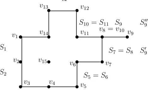
Example: LetV be the set of all dotted grid points in Figure 2.2. C =v1v2v3v4v5v6v7v8v9v10
v11v12v13v14v1 is a contour for V. The condition 3) prevents C0 = v1v2v15v2v3v4v5v6v7
v8v9v10v11v12v13v14v1 from being a contour.
Lemma 9. Let G = (V, EV) be a connected grid graph. If the grid point v ∈ V and grid
point w6∈V have the distance dist(v, w) = 1, then there is a contourC such thatC contains
v and separates w from all grid points of V.
Proof: Imagine that a region starting from the grid point w grows until it touches all of the reachable edges of G(but never crosses any of them). Since Gis a connected grid graph, the boundary forms a contour that consists of edges of G. As dist(w, v) = 1, the vertex v
should appear in the contour.
Lemma 10. Let G= (V, EV) be a grid graph and C be a contour of G. Let
U ={u|u is a grid point not inV withdist(u, v) = 1for some v ∈V and C separates u fromV}.
Then there is a list of grid pointsu1, u2,· · ·, um+1 inU such thatum+1 =u1, dist(ui, ui+1)≤
√
2 for i = 1,2,· · ·, m and all points of P are on one side of the circle path u1u2· · ·um+1
(the edge connecting every two consecutive points u1, u2 is straight line).
Proof: Walking along the contour C =v1· · ·vkv1, we assume that only the left side has
the points from V. A point vi on C is called special point if vi−1 = vi+1. The point v9 is
a special point at the contour v1v2· · ·v14v1 in Figure 2.2. For each edge (vi, vi+1) inC, the
grid square, which is on the right side of (vi, vi+1) and contains (vi, vi+1) as one of the four
boundary edges, has at least one point not inV. Let S1, S2,· · ·, Sk be those grid squares for
(v1, v2),(v2, v3),· · ·,(vk, v1), respectively. For each special point vi on C, it has two special
grid squares S0
i and Si00 that share the edge (vi, u) for some u ∈ U with dist(u, vi) = 1
and dist(u, vi−1) = 2 (for example, S90 and S900 on Figure 2.2). Insert Si0 and Si00 between Si and Si+1. We get a new list of grid squares H1, H2,· · ·, Hm. We claim that for every
two consecutive Hi and Hi+1, there are grid points ui ∈ Hi∩U and ui+1 ∈ Hi+1 ∩U with
dist(ui, ui+1)≤
√
2. The lemma is verified by checking the following cases: Case 1. Hi =Sj and Hi+1 =Sj+1 for some j ≤k.
Subcase 1.1. Sj and Sj+1 share one edge vj+1u. An example of this subcase is the grid
squares S1 and S2 on Figure 2.2. It is easy to see that u ∈ U since u is on the right side
t
v1
S1
S2 t
t
v2 v15t
tv5
S5 =S6
S7 =S8 S90
S00 9
S9
S10 =S11
S12
t
v4 tv3
t
v14 t
v13 tv12
tv11 vt8 =v10 tv9
tv 7 t
v6
Figure 2.2: Contour C =v1v2· · ·v14v1. The node v9 is a special point. When walking along
v1· · ·v14v1, we see that each Si is the grid square on the right of vivi+1
Subcase 1.2. Sj = Sj+1. An example of this subcase is the grid squares S5 and S6 on
Figure 2.2. This is a trivial case.
Subcase 1.3. Sj and Sj+1 only share the point vj+1. An example of this subcase is the
grid squares S11 and S12 on Figure 2.2. We have grid points u1 ∈ U and u2 ∈ U such that
dist(u1, vj+1) = 1, dist(u2, vj+1) = 1. Furthermore, dist(u1, u2) =
√ 2.
Case 2. Hi =Sj00 and Hi+1 =Sj for some j < m. An example of this subcase is the grid
squares S00
9 and S9 on Figure 2.2. The two squares share the edge vju for someu ∈U.
Case 3. Hi =Sj0 and Hi+1 =Sj00. An example of this subcase is the grid squares S90 and
S00
9 on Figure 2.2. The two squares share the edge uju for some u∈U.
Case 4. Hi =Sj−1 and Hi =Sj0. An example of this subcase is the grid squares S8 and
S0
9 on Figure 2.2. The two squares share vju for some u∈U.
Definition 11. For a regionR on the plane, define A(R) to be the area size of R. An unit circle has radius 1. For a region R in the unit circle, L(R) is the length of the boundary of
R inside the internal area of the unit circle. A region R inside a unit circle is type 1 region if part of its boundary is from the unit circle boundary. Otherwise, it is calledtype 2 region, which does not share any boundary with the unit circle.
Lemma 12. Assume s > 0 is a constant and p1, p2 are two points on the plane. We have
1) the area with the shortest boundary and area size s on the plane is a circle with radius
ps
π; and 2) the shortest curve that is through both p1 and p2, and forms an area of size s
with the line segment p1p2 is a circle arc.
circle arc with p1 and p2 as two end points. Let C0 be the rest of the boundary of R. Let
R0 be the region with the boundary C and line segment p
1p2. Assume the length of C0 is
minimal. If A(R) =A(R0), then C0 is the same as the line segment p
1p2. If A(R)< A(R0),
then C0 is a circle arc inside R0 (between C and p
1p2). If A(R) > A(R0), then C0 is also a
circle arc outside R0. Those facts above follow from Lemma 12.
Lemma 13. Let s≤ π be a constant. Let R1, R2,· · ·, Rk be k regions inside an unit circle
(they may have overlaps), Pk
i=1A(Ri) =s and Pki=1L(Ri) is minimal. Then k= 1 and R1
is a type 1 region.
Proof: We consider the regions R1,· · ·, Rk that satisfy Pki=1A(Ri) = s and Pki=1L(Ri)
is minimal for k ≥ 1. Each Ri(i = 1,· · ·, k) is either type 1 or type 2 region. The part of
boundary ofRi that is also the boundary of the unit circle is called old boundary. Otherwise
it is called type new boundary.
A type 2 region has to be a circle (by Lemma 12). For a type 1 region, its new boundary inside the unit circle is also a circle arc (otherwise, its length is not minimal by part 2 of Lemma 12). If we have both type 1 region R1 and type 2 region R2. Move R1 to R1∗ and
R2 to R∗2 on the plane so thatR∗1 and R∗2 have some intersection (not a circle) at their new
boundaries. LetR0
2 be the circle with the same area size asR∗1∩R2∗. The boundary length of
R0
2 is less than that ofR∗1∩R2∗. So,L(R1) +L(R2) reduces to L(R∗1∪R∗2) +L(R02) if R1 and
R2 are replaced byR1∗∪R2∗ andR02 (Notice thatA(R1) +A(R2) =A(R∗1∪R∗2) +A(R∗1∩R∗2) =
A(R∗
1 ∪R2∗) +A(R02)). This contradicts that
Pk
i=1L(Ri) is minimal. Therefore, there is no
type 2 region. We only have type 1 regions left. Assume that R1 and R2 are two type
1 regions. Let R1 and R2 have the unit circle arcs p1p2 and p2p3 respectively. They can
merge into another type 1 region R with the unit circle arc p1p2p3 and the same area size
A(R) = A(R1) +A(R2). Furthermore, L(R) < L(R1) +L(R2). A contradiction again.
Therefore, k = 1 and R1 is a type 1 region.
Definition 14. Let q be a positive real number. Partition the plane into q×q squares by the horizontal lines y = iq and vertical lines x = jq (i, j ∈ Z). Each point (iq, jq) is a (q, q)-grid point, where i, j ∈Z.
Lemma 15. Let V be the set of all (q, q) grid points in the unit circle C. Let G= (V, EV)
be the grid graph on V, where EV = {(vi, vj)|dist(vi, vj) = 1 and vi, vj ∈ V}. Assume that l is a curve that partitions a unit circle C into P1 and P2 with AA((PP12)) = 1t. If the minimal
length of l is c0, then every t -separator for the grid graph G has a size ≥ c0( √
n−√2π)
Proof: Assume that the unit circleC area hasn(q, q)-grid points. We haveπ(1+q√2)2 ≥
n·q2. It implies q ≤ 1
√n
√π−√2.Assume A⊆V is the smallest separator for G= (V, EV) such thatG−Ahas two disconnected subgraphsG1 = (V1, EV1) andG2 = (V2, EV2), which satisfy
|V1|,|V2| ≤ ttn+1. By Corollary 6,|A| ≤2√n. LetG1 have connected componentsF1,· · ·, Fm.
By Lemma 10, each Fi is surrounded by a circular path Hi with grid points not from G1.
Actually, the grid points ofHiinsideC are from the separatorA. LetP1,· · ·, Pk be the parts
of H1,· · ·, Hm inside the C. They consist of vertices in A and the distance between every
two consecutive vertices in each Pi is≤
√
2q (by Lemma 10 and scaling (q, q) grid points to (1,1) grid points).
The number of (q, q)-grid points with distance ≤ 2 to the unit circle boundary is also
O(√n). For a (q, q)-grid point p = (iq, jq), define gridq(p) = {(x, y)|iq − q2 ≤ x ≤ iq +
q
2 and jq −
q
2 ≤ y ≤ jq +
q
2}. Let VH be the set of all (q, q)-grid points in H1,· · ·, Hm
and VP be the set of all (q, q)-grid points in P1,· · ·, Pk. Let S1 = ∪p∈V1gridq(p), S10 =
∪p∈V1∪VHgridq(p), and S100 = ∪p∈V1∪VPgridq(p). It is easy to see that
2n
3q2 ≥ A(S1) ≥
n
3q2
and A(S0
1) = A(S1) +O(√n) and A(S100) = A(S1) +O(√n). Therefore, the sizes of S10 and
S00
1 are almost the same as that of S1 (because √n << n). For the variable x ≥ 1, define
the function g(x) to be the length of the shortest curve that partitions the unit circle into regions P1 and P2 with AA((PP21)) = x1. Then g(x) is a decreasing continuous function (see the
analysis in section 2.4).
The total length of P1,· · ·, Pk is minimal when k= 1 by Lemma 13. Since the length of P1 is ≥c0, there are at least qc√02 ≥
c0(
√n √π−√2)
√
2 =
c0(√n−
√ 2π) √
2√π grid points of A along P1.
Theorem 16. There exists a grid graph G= (V, EV) such that for anyA ⊆V if G−A has
two disconnected graphs G1 and G2, and Gi(i= 1,2)has ≤ 2|3V| nodes, then|A| ≥0.7555√n
when n is large.
Proof: By Theorem 17 in the next section, the length of the shortest curve partitioning the unit circle into 1 : 2 ratio is ≥ 1.8937. By Lemma 15 with c0 = 1.8937 and k = 1, we
have |A| ≥0.7555√n.
2.4.
Shortest separator of the unit circle
that the ratio A1/A2 of the two pieces is a constant k. The length of the curve connecting the two fixed points is the functional expression
L(x, f(x), f0(x)) =
x2
Z
x1
p
1 + (f0(x))2dx, (2.5)
where prime denotes the derivative with respect to x. The constant ratio of the two areas
A1/A2 =k, together with A1+A2 =πR2, gives A1 =πR2k+1k . To determine the extremum
of the functional (2.5) with the above constraint on A1, we used the Lagrange multipliers
method (see [56]). The functional whose extremum we are searching for is
L∗(x, f(x), f0(x)) = L(x, f(x), f0(x)) +λ
A1−πR2
k k+ 1
= (2.6)
=
x2
Z
x1
p
1 + (f0(x))2dx+λ
x2
Z
x1
√
R2−x2−f(x)dx−πR2 k
k+ 1
,
where λ is the Lagrange multiplier and A1 =
x2
R
x1
√
R2−x2−f(x)
dx (Figure 2.3A).
The functional that determines the extremum of (2.6) isF(x, f(x), f0(x)) =p1 + (f0(x))2+
λ √R2−x2−f(x)
. The Euler-Lagrange equation of the functional F(x, f(x), f0(x)) is
∂F ∂f −
d dx
∂F
∂f0 = 0. The solution of the Euler-Lagrange equation is the minimum length
sepa-rator function y=f(x) with
f(x) =b−
s
1
λ
2
−x+ a
λ
2
, (2.7)
wherebis an arbitrary constant. The solution (2.7) of the variational problem (2.6) represents a circle of radius r = 1
λ and center at (− a
λ, b) (Figure 2.3B, C).
The area of the circular region subtended by the angle θ isR2(θ−sin(θ))/2, and by the
angle φ is r2(φ−sin(φ))/2 (Figure 2.3B). Therefore, the total area A
1 is given be the sum
of the above areas
A1 =
R2
2 (θ−sin(θ)) +
r2
2(φ−sin(φ)) =πR
2 k
x y
R (x ,y )
(x ,y ) 1 2 1 2 A1 2 A A θ x y
(-x ,y )1 1 (x ,y )1 1
R
φ
φ
π/4 π/2 3π/4 π
1.1 1.0 0.95 1.05
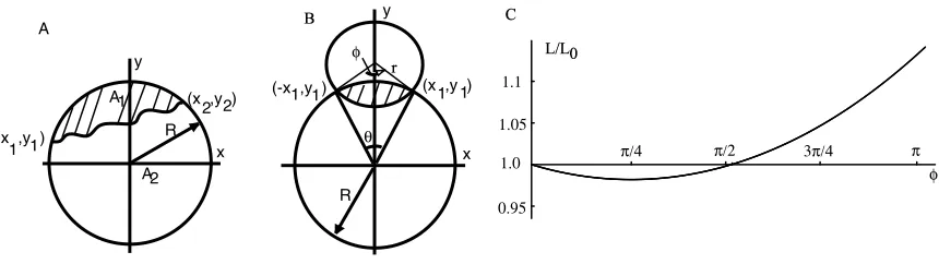
Figure 2.3: The minimum length path that divides a circle into two regions with a fixed ratio k. A. The minimum length curve connecting the points (x1, y1) and (x2, y2) is the
solution of the variational problem (2.6). B. The solution of the variational problem is a circle of radius r with a subtending angle φ < π. C. Implicit plot of the normalized arc length L/L0 versus the subtended angle φ. For k = 1/2 the arc has a minimum length
Lmin ≈0.982002L0 = 1.8937 for an angle φmin ≈0.79388.
with the additional obvious relationship (Figure 2.3B)
Rsin(θ/2) =rsin(φ/2). (2.9)
The length of the separator arc that connects the two points (−x1, y1) and (x1, y1) on the
circle of radius r is L=rφ (Figure 2.3B). By substituting the explicit expression ofθ from (2.9) into (2.8), we get an implicit relationship between the variables r and φ
2 arcsin r R sin φ 2 −sin 2 arcsin r Rsin φ 2 + r 2
R2(φ−sin(φ)) = 2π
k
k+ 1. (2.10)
Using the definition of the arc length we getr=L/φ, which substituted into (2.10) leads to an implicit relationship between the arc lengthL and the subtending angle φ
2 arcsin L Rφsin φ 2 −sin 2 arcsin L Rφsin φ 2 + L 2
R2φ2(φ−sin(φ)) = 2π
k
k+ 1. (2.11)
We numerically solved the implicit equation (2.11) for different values of φ ∈ (0, π) (Fig-ure 2.3C). The arc lengthLwas normalized by the arc lengthL0 of the straight line that cuts
the circle of radius R with the same ratio k =A1/A2 (Figure 2.3A). Based on Figure 2.3B,
the lengthL0 of the straight line that cuts the circle in two regions with the given ratiok is
L0 = 2Rsin θ20
. The angle θ0 is the solution of the constraint equation (2.8) in the limit
(R = 1) and k = 1/2 the numeric solution is θ0 ≈ 2.60533 radians, and the corresponding
length of the straight line separator is L0 ≈1.92853.
We numerically found that the arc separator measured along the circle of radius r is always shorter than the corresponding straight line separator (L/L0 ≤1) if the subtending
angle φ ∈ (0, π/2) (Figure 2.3C). If the subtending angle φ < π/2 (Figure 2.3B, C), then there is a value,φmin, such that the arc length is the minimum possible and this is the optimal
solution for the separator length. We numerically found thatφmin ≈0.79388∈(0, π/2) and
the corresponding radius of the circle is r ≈ 1.23672R. If the subtending angle φ > π/2, according to the numerical solution of the implicit equation (2.11) shown in (Figure 2.3C), the arc is no longer the minimum length solution of the variational problem. We formulate our analysis to the theorem below:
C
ha
pter
3
Application of multi-directional
width-bounded geometric separators
to protein folding in the HP model
We have shown that there is a sizeO(√n) separator line to partition the folding problem ofn
letters into 2 problems in a balanced way. The 2 smaller problems are recursively solved and their solutions are merged to derive the solution to the original problem. As the separator has onlyO(√n) letters, there are at most nO(√n) cases to partition the problem. The major
improvement from the algorithm in [27] is the approximation of the optimal separator line. We need the following terms:
Definition 18.
• For integers i and j, integer interval [i, j] = {i, i+ 1,· · ·, j}. For a set Σ of letters, a Σ-sequenceis a sequence of letters from Σ. For example,P HP P HHP H is an{H, P} -sequence. For a sequence S of length n and 1 ≤ i ≤ n, S[i] is the i-th letter of
S. S[i, j] denotes the subsequence S[i]S[i+ 1]· · ·S[j]. If [i1, j1],[i2, j2],· · ·,[it, jt] are
disjoint intervals inside [1, n], we callS[i1, j1], S[i2, j2],· · ·, S[it, jt]disjoint subsequences
of S. For a set of integers A={i1 < i2 <· · ·< ik}, define S[A] =S[i1]S[i2]· · ·S[ik].
• For a 2-dimensional point (x1, x2), define ||(x1, x2)||=|x1|+|x2|.
• A self-avoiding arrangementf for a sequence S of length n on the 2-dimensional grid is a one-to-one mapping from {1,2,· · ·, n} to Z2 such that ||f(i)−f(i+ 1)|| = 1 for
self-avoiding arrangement of S on S[i1, j1],· · ·, S[ik, jk] is a partial function f from
{1,2,· · ·, n} to Z2 such that f is defined on ∪k
t=1[it, jt], and f can be extended to a
(full) self-avoiding arrangement of S onZ2.
• For a grid self-avoiding arrangement, itscontact mapis the graphGf = (1,2,· · ·, n, E),
where the edge set E ={(i, j) :|i−j|>1 and ||f(i)−f(j)||= 1}.
• For a lineLwith equationf(x, y) = 0, defineL<0 andL>0 as the area{(x, y)|f(x, y)<
0} and {(x, y)|f(x, y)>0} respectively.
Assume that our input HP sequence has n0 letters and the optimal folding is inside an
m×m square. We will select a parameter0 >0. Add some points evenly on the four edges
of the m×m square, so that every two neighbor points on the same line of the boundary have distance 0. Those points are called 0-regular points. Every line segment connecting
two 0-regular points is called a 0-regular line segment. A 0-regular line is a line containing
two 0-regular points.
Lemma 19. Let m > 2. Let 1 > > 0 and δ > 0 be two small constants. Let c1 be a
constant > (1+3)2. Let L be a line, which intersects the m×m square A and has the slope
s. The four boundary lines segments of A are either vertical or horizontal. Each side of
L has ≥ c1 grid points in A and ≤ |s| ≤ 1. Then for some constant c2 > 0 and every
0 < 0 ≤ 1
c2·m, there exists an
0-regular line L0 such that for every grid point q ∈ A with
≤(a, a) to L0 has ≤(a+δ, a+δ) distance to L.
Proof: LetV1 andV2 be the two line segments of vertical boundary ofA. Let H1 and H2
be the two line segments of the horizontal boundary ofA. Let p1 = (x1, y1) andp2 = (x2, y2)
be the two intersections of L with the boundary of A. Let p0
1 = (x01, y01) and p02 = (x2, y2)0
be the two closest 0-regular points to p
1 and p2 respectively on the boundary of A, where 0
will be determined later. Let q= (x0, y0) be a grid point in A. Let L0 be the 0-regular line
through both (x0
1, y10) and (x02, y20).
Let Lv and Lh be the vertical and horizontal lines through q, respectively. The
intersec-tion betweenLandLh is at the point (x, y0), where x= xy22−−xy11(y0−y1) +x1. The intersection
between L and Lv is at the point (x0, y), where y = xy20−−yx11(x0−x1) +y1.
Similarly, the intersection betweenL0 andL
h is at the point (x0, y0) wherex0 = x
0
2−x01
y0
2−y01(y0−
y0
1) +x01. The intersection between L0 and Lv is at the point (x0, y0), where y0 = y
0
2−y01
x0−x01(x0 −
have s= y2−y1
x2−x1. The line L
0, which is through (x0
1, y10) and (x02, y20), has the slopes0 =
y20−y01
x0
2−x01.
By the condition of this lemma, we have
≤ |s|=
y2−y1
x2−x1
≤ 1 . (3.1)
Case 1: bothp1 andp2are inV1∪V2. This implies that|x2−x1|=m. Since|s|=|xy22−−xy11| ≥,
we have |y2−y1| ≥m.
Case 2: both p1 and p2 are in H1 ∪H2. This implies that |y2 −y1| = m. Since |s| =
|y2−y1
x2−x1| ≤
1
, we have |x2−x1| ≥m.
Case 3: p1 and p2 are inVi∪Hj for somei, j. We have (|x2−x1|+ 2)(|y2−y1|+ 2)≥c1
since each side ofLhas at leastc1grid points inA. Then (|x2−x1|+2)(|x2−x1|+2) > c1. This
gives that |x2−x1| > √
4c1+4+4−(2+2)
2 >
√c
1−(1 +). Since √c1 ≥
q
(1+3)2 = 1 + 3, |x1−x2| ≥√c1 −(1 +)≥1 + 3−(1 +)≥2. Similarly, |y2−y1|>2. Combining the
cases 1 to 3, we always have
|x1−x2| ≥2 and |y1−y2| ≥2. (3.2)
Letx0
2−x01 =x2−x1+x andy20−y10 =y2−y1+y. Since (x01, y10) is the closest0-regular
point to (x1, y1) and (x02, y02) is the closest0-regular point to (x02, y20),|x| ≤20 and|y| ≤20.
Define
0,s =
40
2 (3.3)
|s−s0| =
y2−y1
x2−x1 −
y0 2−y10
x0 2−x01
=
(y2−y1)(x02−x01)−(y20 −y01)(x2−x1)
(x2−x1)(x02−x01)
=
(y2−y1)(x2−x1+x)−(y2−y1+y)(x2−x1)
(x2−x1)(x2−x1+x)
=
(y2−y1)x−y(x2 −x1)
(x2−x1)(x2−x1+x)
=
x(y2−y1)
(x2−x1)(x2−x1+x) −
y
(x2−x1 +x)
≤
|x||s|
|x2−x1+x|
+ |y|
|x2 −x1+x|
≤ x
(x2−x1+x)
+ y
|x1−x2| − |x|
≤
20
2 +
20
≤
40
2 =0,s. (3.4)
For (3.4) to (3.4), it is because |x1−x2| − |x| ≥2−≥ by (3.2). Let x01 =x1+1,x, y0
1 =y1+1,y and s0 =s+s. By (3.4) to (3.4), we have the inequality:
Since (x0
1, y01) is the closest 0-regular point to (x1, y1) and (x02, y20) is the closest 0-regular
point to (x0
2, y20), |1,x| ≤ 0 and |1,y| ≤ 0. We consider the difference between y and y0 as
well as the difference between xand x0.
|y−y0| = |(s(x0−x1) +y1)−(s0(x0−x01) +y10)|
= |(s(x0−x1) +y1)−((s+s)(x0−x1−1,x) +y1+1,y)|
= | −(x0−x1)s+1,x(s+s)−1,y|
≤ |(x0−x1)s|+|1,x(s+s)|+|1,y|
≤ |s|m+
1,x(
1
+|s|)
+|1,y| ≤ |s|m+
21,x
+|1,y|. (3.6)
For (3.6) → (3.6), it is because the following facts: By (3.3) and (3.5), |s| ≤ |0,s| ≤
40
2 ≤ 12 ≤ 1 (the condition 40 ≤1 will be satisfied when we set the constant 0 later).
|x−x0| = 1
s(y0−y1) +x1
−
1
s0(y0−y 0 1) +x01
= 1
s(y0−y1)−
1
s+s
(y0−y1−1,y)−1,x
=
(y0−y1)(
s s(s+s)
) + 1,y
s+s − 1,x ≤
(y0−y1)(
s s(s+s)
) + 1,y s+s
+|1,x|
≤
n( s
s(s+s)
) + 1,y s+s
+|1,x| ≤
n(2s
2 ) +
21,y
+|1,x|. (3.7)
For (3.7)→(3.7), it is because the following facts: By (3.5),|s| ≤0,s = 4
0
2 ≤ 2 (we will set
up 0 so that 0 ≤ 3
8). This implies that |s+s| ≥ |−
2| ≥
2. Therefore, |s(s+s)| ≥
2
2.
We choose 0 so that it satisfies the following inequalities: (1)|
s|m ≤ δ3, (2)
21,x
≤ δ 3,
(3)|1,y| ≤ 3δ, (4) |m(2s)| ≤ δ3, (5)|
21,y
| ≤ δ
3, (6)|1,x| ≤
δ
3, (7)40 ≤ 1, and (8) 0 ≤
3
8. Let
e0 ≤min( δ2
12m, δ
6,
δ
6,
δ4
12m, δ 6, δ 6, 2, 1 4, 3
8), in which each item is for the corresponding condition
among (1)-(8). We let 0 = δ4
12m, which makes both |x−x0| ≤ δ
3 +
δ
3 +
δ
3 =δ and |y−y0| ≤
δ
3 +
δ
3 +
δ
3 =δ.
Lemma 20. Let a and δ be positive constants. Let P be a set of n grid points in a 2-dimensional m×m square. There exist 0 = 1
c02m and 0-regular line L0 such that there are
≤(23 +δ)n points of P on each half plane (divided by L0), and ≤k
0a(1 +δ)√n points of P
with distance ≤(a, a) to L0 for all large n, where k