Xu et al. Carbon Balance Manage (2016) 11:18
DOI 10.1186/s13021-016-0062-9
RESEARCH
Performance of non-parametric
algorithms for spatial mapping of tropical forest
structure
Liang Xu
1*, Sassan S. Saatchi
1,2, Yan Yang
1,3, Yifan Yu
2and Lee White
4Abstract
Background: Mapping tropical forest structure is a critical requirement for accurate estimation of emissions and removals from land use activities. With the availability of a wide range of remote sensing imagery of vegetation characteristics from space, development of finer resolution and more accurate maps has advanced in recent years. However, the mapping accuracy relies heavily on the quality of input layers, the algorithm chosen, and the size and quality of inventory samples for calibration and validation.
Results: By using airborne lidar data as the “truth” and focusing on the mean canopy height (MCH) as a key structural parameter, we test two commonly-used non-parametric techniques of maximum entropy (ME) and random forest (RF) for developing maps over a study site in Central Gabon. Results of mapping show that both approaches have improved accuracy with more input layers in mapping canopy height at 100 m (1-ha) pixels. The bias-corrected spatial models further improve estimates for small and large trees across the tails of height distributions with a trade-off in increasing overall mean squared error that can be readily compensated by increasing the sample size.
Conclusions: A significant improvement in tropical forest mapping can be achieved by weighting the number of inventory samples against the choice of image layers and the non-parametric algorithms. Without future satellite observations with better sensitivity to forest biomass, the maps based on existing data will remain slightly biased towards the mean of the distribution and under and over estimating the upper and lower tails of the distribution.
Keywords: Tropical forests, Canopy height, Lidar, Spatial mapping, Gabon
© 2016 The Author(s). This article is distributed under the terms of the Creative Commons Attribution 4.0 International License (http://creativecommons.org/licenses/by/4.0/), which permits unrestricted use, distribution, and reproduction in any medium, provided you give appropriate credit to the original author(s) and the source, provide a link to the Creative Commons license, and indicate if changes were made.
Background
Structure and aboveground biomass (AGB) of tropical forests are highly variable, creating landscape scale heter-ogeneity that cannot be readily captured without spatial mapping or increasingly dense systematic sampling [1– 3]. The uncertainty in the distribution of AGB and forest structure at local to regional scales has impacted the esti-mation of greenhouse gas (GHG) emissions and remov-als from land use activities [4, 5], the monitoring of the global carbon cycle [6], and the development of climate change mitigation policies in the framework of REDD (reduced emissions from deforestation and degradation)
[7]. Local and landscape heterogeneity of tropical forest biomass and structure are larger than regional and conti-nental scale variations [1, 8–11], making extrapolation or estimation of finer scale variations difficult and uncertain [2].
Increasing availability of airborne observations of trop-ical forests with Lidar and radar remote sensing tech-niques, has significantly improved our ability to quantify and map forest structure at higher spatial resolution [12–15]. Unlike conventional passive optical sensors, these active sensors can capture the vertical vegetation structure by either measuring the range of laser light reflected from vegetation elements and the ground [16, 17], or measuring the radar backscatter and phase at a given wavelength and polarization [15, 18–20]. Among these new techniques, high resolution (small footprint)
Open Access
*Correspondence: [email protected]
1 Institute of the Environment and Sustainability, University of California, Los Angeles, CA 90095, USA
the non-parametric algorithm that is used as an estima-tor of forest structure for each mapping unit or pixel, the quality of satellite imagery and the environmental varia-bles, and the quality and quantity of samples used to train the non-parametric models [24].
The Lidar-derived metric, mean canopy height (MCH), or the centroid of the vertical canopy profile [25], has been found to be the best variable calibrating AGB as a single-metric model [21, 26]. Although MCH may under-estimate the canopy heights in complex terrain under the circumstance of reduced data density [27], it has excellent agreements with field-measured maximum and mean tree heights at least in low-slope environments [28] as well as the field-measured basal area [29]. However, air-borne Lidar still exists as a sampling tool in most regions of the tropics, because the wall-to-wall Lidar data are scarce. For large-scale mapping, airborne/satellite Lidar is sampled as a surrogate for tropical forest structure and use radar and optical imagery for spatial modeling and mapping [12, 15, 30–32]. In mapping forest structure at medium-to-high resolution (e.g. 100-m), high-qual-ity satellite data include the Landsat series in the opti-cal domain, the L-band radar backscatter data collected from the Advanced Land Observing Satellite “DAICHI” (ALOS) platform and the digital elevation model (DEM) data derived from the Shuttle Radar Topography Mission (SRTM) in the microwave domain. The accuracy of the maps depends strongly on the quality and relevance of satellite input layers, the model setup suitable for tropi-cal forest structure prediction, as well as the design and selection of the training samples.
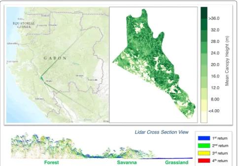
In this study, we utilize small footprint airborne lidar data to evaluate the performance of high-resolution map-ping of tropical forest structure from satellite layers using popular machine learning algorithms. The study area is located north of the City of Mouila in Ngounie prov-ince in southwestern Gabon, covering approximately 33,500 ha of moist tropical forests and savanna west of Ngounie river. Gabon is the second most forested coun-try in the world after Surinam, with 85 % (24,000 km2)
of its area (267,667 km2) covered by tropical
rainfor-est [15]. The area selected for this study is relatively flat with approximately 40 m variations in elevation from
was measured by airborne lidar for carbon assessment (Fig. 1).
Given the fact that Lidar-derived MCH can act as the ground (airborne) truth representing forest structure and carbon stocks with only a few field plots to stabilize [21, 23], we focus on MCH mapping from satellite data using a small number of training samples. Through the use of non-parametric models, the random forest (RF) and the Maximum Entropy (ME) algorithms, we try to answer the following questions: (1) What types of infor-mation should be included as input layers to improve the model predictions? (2) How can we adjust the learning algorithms to suit our needs for unbiased estimations, especially for large trees? (3) What is the effectiveness of forest structure mapping from current satellite data using a limited quantity of ground measurements? For regional-scale analyses, sampling strategy is one of the key components for successful mapping of forest struc-ture. The continuous coverage of Lidar-derived MCH gives us the opportunity to showcase a set of benchmark tests of satellite retrievals for forest structure and carbon stocks using empirical (machine learning) methods. We expect these results can serve as guidelines for parame-ter tunings of machine learning algorithms dedicated to tropical forest structure retrievals, and also help to better design future field plots at local to regional scales.
Results and discussion
Passive optical, radar backscatter, interferometry, and texture information
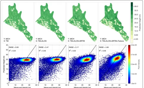
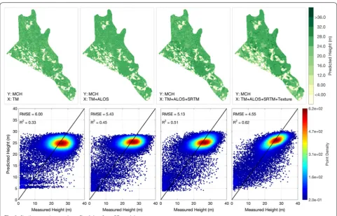
Using default settings of both RF and ME algorithms, we tested the MCH prediction capability of Landsat, ALOS and SRTM in 100-m spatial resolution, and found improved predictions of MCH when adding more infor-mation from different satellite layers (Figs. 2, 3). Both algorithms produce similar prediction accuracy regard-ing root-mean-square error (RMSE) or coefficient of determination (R2). By conducting Monte Carlo cross
validations (CV), the RMSE of RF method decreases from 6.02 ± 0.10 m (predicted from Landsat data alone) to 5.06 ± 0.07 m when using all inputs from three sat-ellite sensors (Table 1). R2 values have an
Page 3 of 14 Xu et al. Carbon Balance Manage (2016) 11:18
have a comparable RMSE (R2) accuracy, starting from
6.00 ± 0.10 m (R2 = 0.34 ± 0.02) for Landsat only
predic-tions, to 5.17 ± 0.09 m (R2 = 0.52 ± 0.01) for predictions
from all three sensors. Tests using data from each satel-lite sensor show similar prediction accuracies (Table 1), with ALOS being the most sensitive to MCH, but none of them has the comparative prediction power of all sensors combined. The significant improvements with the addi-tion of layers suggest that the data fusion from different sensors can help to achieve better prediction results.
However, neither model shows an unbiased prediction along the one-to-one line of the actual MCH values. The scatter plots of test data (lower panels in Figs. 2, 3) show a vast majority of predictions around 25 m, thus having a flattened oval shape along the X-axis. This pattern of deviation from the one-to-one line means an underesti-mation of high MCH and an overestiunderesti-mation of low MCH. Although the overall mean signed deviation (MSD) is small when calculated from all test points, the MSD for large trees (MSD2) reveals a significant underestimation that is consistently lower than the measured MCH by
5–10 m. But this quantity also improves with increased number of input layers, meaning the extra information provided by additional layers increases the sensitivity of input signal to large trees. Similarly, the MSD for small trees (MSD1) has an overestimation of 4–6 m, and it does not improve much with more input layers.
In addition to the original input bands from satellite observations at corresponding locations, we also tested the contribution of surrounding pixels to the MCH prediction. Both RF and ME prediction results show a further improvement when adding texture layers (last column of Figs. 2, 3). The texture information brings an additional half meter decrease in RMSE for the RF results (0.44-m decrease for ME), and improves the R2 by 0.1
(0.07 for ME) (Table 1). Another important contribution of adding texture is making the predictions less biased. There are much more pixels with predicted MCH over 30 m, compared to the predictions without texture. The red oval, representing the majority of test data in the scatter plot (Figs. 2, 3), also reclines more toward the one-to-one line of MCH. Although it does not change a lot on
the overall MSD, which is always unbiased, the MSD2 appears to be less biased (−5.16 m for RF, and −4.39 for ME).
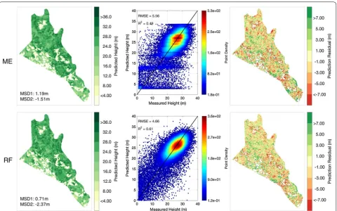
Model adjustments dedicated to tropical forests
Unbiased estimation of large trees is important in the structure retrieval of tropical forests, as they are the dominant component in biomass and carbon stocks. Bias correction is, therefore, the major task of the model adjustment in tropical forests. Results of ME adopting the published tuning method [15, 34] will reduce the bias at the cost of more dispersed predictions, i.e., larger RMSE and smaller R2 values (Fig. 4). Using the same
set-tings of training and test samples, the bias-corrected ME (MEBC) shows significant reductions in MSD1 from 4.57 to 1.10 m, and MSD2 from −4.39 to −1.13 m (Table 1). However, MEBC loses accuracies in RMSE and R2 (RMSE
from 4.7 to 5.3, and R2 from 0.59 to 0.53) as an adverse
effect of bias correction.
The application of the bias correction method on the RF results in similar prediction accuracy as the original RF with a significant improvement in MSD1 and MSD2. The Monte Carlo CV results also indicate that this improve-ment is not a coincidence from a single realization
(Table 1). The bias-corrected version of RF (RFBC) has comparable R2 as the original RF (0.63 ± 0.01), a slightly
larger RMSE (4.60 m), and a significantly reduced MSD1 from 4.5 to 0.7 m, and MSD2 from −5.4 to −1.7 m.
Effects of sample size
It is well known that increasing the training sample size can help to improve the prediction accuracies, but it is unclear whether the improvements in MSD using the bias-corrected methods can also be achieved by increas-ing the sample size usincreas-ing original methods. Alternatively, it is important to test whether the sample size increase can compensate the losses in RMSE and R2 when using
bias-corrected methods.
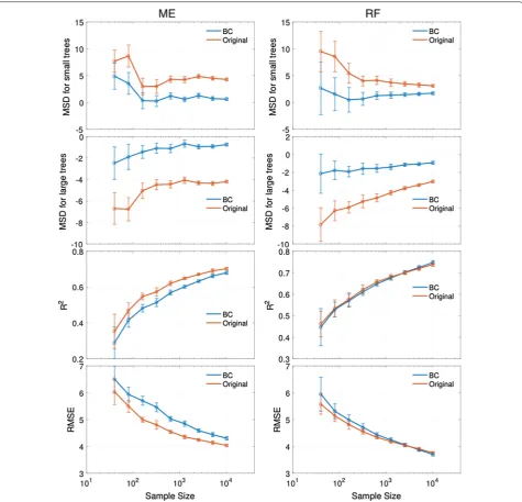
Monte Carlo CV tests (Fig. 5) comparing RF and RFBC show that for sample size up to ten thousand (around one-third of all valid observations), the original RF can never achieve the same level of MSD2 (around −2 m) by using RFBC, even when RFBC has only 40 training sam-ples. MSD1 from RFBC also shows consistently lower biases than what we get from the original RF model. Meanwhile, RF and RFBC results have very similar R2
values across all sample sizes, and RFBC has a slightly larger RMSE than the original RF when the sample size
Page 5 of 14 Xu et al. Carbon Balance Manage (2016) 11:18
is below 2500. The result suggests that predictions using RFBC can always achieve the same level of accuracy by increasing the sample size. For example, on average there is a 0.2-m difference in RMSE between using RF and
using RFBC when we have 80 training samples, but this lower RMSE obtained from RFBC can be easily improved by adding around 30–40 training samples. A more inter-esting finding of RFBC is that the accuracy exceeds the
Fig. 3 Similar mapping results as Fig. 2, but from RF models
Table 1 Machine learning performance using different input layers
The sample size for this test was fixed at 400 samples, and the rest 32,674 100-m pixels were used as test samples. The results were cross validated by repeated random sampling of the training data (Monte Carlo CV). RF and ME predictions were evaluated using RMSE, R2, overall MSD, MSD for small trees (MSD1) and the MSD
for large trees (MSD2). The input “L only” includes four Landsat bands, “A only” uses only the two ALOS bands, “S only” uses only the SRTM bands, “L + A” includes four Landsat and two ALOS bands, “L + A + S” includes Landsat, ALOS and SRTM bands, “L + A + S + T” includes all satellite bands plus texture layers, and “BC” uses the same set of input layers as “L + A + S + T”, but results are from the bias-corrected algorithms
Input layers L only A only S only L + A L + A + S L + A + S + T BC
RF
RMSE 6.02 ± 0.10 5.80 ± 0.08 6.20 ± 0.04 5.41 ± 0.07 5.06 ± 0.07 4.51 ± 0.07 4.58 ± 0.09 R2 0.33 ± 0.02 0.39 ± 0.02 0.30 ± 0.01 0.46 ± 0.01 0.53 ± 0.01 0.63 ± 0.01 0.63 ± 0.01 MSD 0.08 ± 0.23 −0.13 ± 0.33 −0.16 ± 0.31 0.10 ± 0.22 0.12 ± 0.22 0.08 ± 0.25 −0.08 ± 0.18 MSD1 3.68 ± 1.20 2.32 ± 1.15 6.84 ± 1.25 3.80 ± 1.21 3.89 ± 1.24 4.48 ± 0.99 0.71 ± 0.81 MSD2 −8.50 ± 0.45 −7.63 ± 0.60 −7.03 ± 0.81 −7.46 ± 0.50 −5.61 ± 0.59 −5.16 ± 0.43 −1.73 ± 0.57 ME
original RF in all statistical metrics when the sample size is large enough (greater than 2500), suggesting that our proposed bias correction of RF is an overall better model compared to the original for large sample size.
ME results also provide better predictions in MSD1 and MSD2 (Fig. 5), but regarding R2 or RMSE, MEBC
approach needs more training samples to achieve the same accuracy of ME. Using the same example of the sample size of 80, a half-meter difference in RMSE between ME and MEBC predictions requires about 200 additional training samples to amend the RMSE loss. This is practically not cost-effective when considering all the efforts required for the ground data acquisitions and logistics in tropical forests.
Spatial autocorrelation
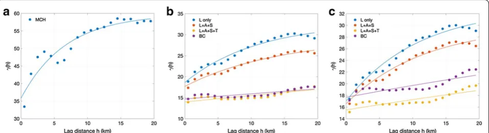
Spatial autocorrelation exists when the value of a pixel is predictable from nearby pixels. Although tropical for-ests are usually dense and heterogeneous, spatial pat-terns are not completely random, and the variogram plot of measured MCH confirms spatial dependence on horizontal distance (Fig. 6a). Previous studies have shown that estimations from sampling data without consider-ing spatial information could introduce large biases and
erroneous spatial representations [1, 2], and thus system-atic sampling from remote sensing data is crucial to the accurate mapping of tropical forests at the regional scale. We also found that the geolocation information aids to improve the remote sensing based predictions substan-tially, assuming that spatial autocorrelations can explain the model residuals. Spatial autocorrelation information can be either modeled through the variance–covariance structure of regression residual in Kriging methods [35] or directly included as another set of predictor variables [24].
In our study, we assumed that the information relating to spatial context could be estimated from surrounding satellite data or texture information, due to the existence of spatial autocorrelation [3, 9]. Texture derived from satellite data is important for high-resolution mapping as it brings additional spatial information for estimating the forest structure from the knowledge of surround-ing pixels. The model prediction improvements were significant when adding texture layers (e.g. Table 1; Figs. 2, 3). From the variogram plots (Fig. 6b, c) show-ing the variance along the paired distance, we also found the flattened slope of semi-variogram for predictions with texture information, suggesting that a large part of
Page 7 of 14 Xu et al. Carbon Balance Manage (2016) 11:18
spatial dependence at the short distance were explained by the texture layers included in the model. The vari-ogram slopes derived from BC model residuals do not differ much from the original models, indicating that the algorithm tuning for bias correction has no significant impact on the spatial autocorrelation.
Comparison of model performance
The performance of original spatial models is approxi-mately the same on the average. However, when they are
tuned to predict the height of tropical forests over the entire range, there are differences when comparing the results on pixel-by-pixels. These differences include (1) a slightly higher bias in RF results towards the mean of samples, reducing the variability in pixels at the tails of the distribution compared to ME. After the bias correc-tion, the difference between RF and ME results still show slight overestimations of RF model in areas with low values and underestimation in areas of high values (e.g. see MSD1 and MSD2 values in Fig. 5). This is due to the
differences between RF and ME algorithms. In MEBC, we simply assign more weights on the most probable classes for correcting biases [15, 34], while in RFBC, we build a second RF model to estimate the biases gener-ated from the original RF model. (2) RF provides much higher prediction accuracy over pixels used for training data compared to the test data, whereas the ME predic-tions showed similar accuracy on both training and test data, suggesting the high dependence on training data in RF models. Although the RF methodology is designed to avoid overfitting [36], there are indications that it tends to capture mistakes in training for small sample size [37]. In contrast, ME methodology avoids overfitting by rely-ing on a regularization technique and a Bayesian estima-tor that includes the prior probability distributions of both training and predictions. (3) For implementation, both techniques have similar computing time and will benefit from parallel processing when used with high-resolution data and multiple layers. Unlike the random forest, the maximum entropy model is designed to work with sub-optimum sample size as it predicts the distri-bution when it is under-sampled as in most signal pro-cessing problems [38]. When the sample size is large compared to the background layers, the ME methodol-ogy may produce additional uncertainty from the over-sampling. This problem may not occur in random forest. This feature also suggests that the ME algorithm may be more suitable in cases where the number of ground sam-ples is limited and small compared to the overall size of the mapping area.
Residual bias
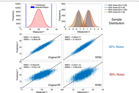
The bias-corrected models of RF and ME both show significant improvements regarding MSDs for small and large trees. However, small biases remain in the prediction residuals even when the sample size is large enough. For example, we still have MSD1 of around 1 m
and MSD2 of −1 m when the RFBC model is trained using 5000 samples. Tests using simulated data with random noise generated in both predictor and response variables show that RFBC has an unbiased estimation for both MSD1 and MSD 2 with a slightly larger disper-sion (RMSE or R2) than the original RF (20 % noise
sim-ulations in Fig. 7). If we generate a simulated dataset with larger noise, i.e., losing sensitivity to the response variable (80 % noise simulations in Fig. 7), both RF and RFBC have less accurate predictions as expected, and importantly, the proposed RFBC method cannot restore the unbiased predictions at both ends. There-fore, the remaining biases could come from sources of errors that are comparable to the signal itself, and thus hard to model or correct. This is particularly true in the case of tropical forests, as both radar and optical obser-vations lose their sensitivity to dense forests and high biomass. The signal-to-noise ratio is very low in these types of forests, causing more estimations towards the mean value. The source of noise could be the effect of environmental conditions in the case of radar data, resulting in high backscatter in low density forests due to the effect of moisture level. The noise in optical data could come from the variations of leaf-level albedo and orientation that significantly alters the canopy-level reflectance, despite the strong impact from can-opy structure. Additional effects of multiple scattering events and speckle noise within and between pixels can further blur the signal of forest structure contained in the satellite data.
Conclusions
Using the tropical forest site in Mouila, Gabon as a case study, we explored the performance of spatial modeling under various circumstances. In particular, we investi-gated the structure retrieval capability using existing sat-ellite imagery with limited sensitivity to forest structure
Page 9 of 14 Xu et al. Carbon Balance Manage (2016) 11:18
variations. Using MCH as the variable of interest and airborne lidar measurements as the surrogate truth, we found: (1) The quality of retrieval improves with more information brought by additional satellite measure-ments and spatial texture layers. (2) The model adjust-ment for bias correction significantly improves the predictions for two edges (small and large trees). And (3) the loss of accuracy in RMSE or R2 due to bias correction
algorithms can potentially be compensated by increasing the sample size of the training data.
With the current level of information and measure-ment errors obtained from remote sensing data, a certain amount of uncertainty in the final product of vegeta-tion mapping is unavoidable, but our study shows that the mapping process can be optimized by considering the choice of inputs, the algorithms to use and the size of samples. With a focus on remote sensing data used in mapping tropical forest structure, we expect this study will help to utilize the existing machine learning algo-rithms better and modify them appropriately to suit the needs for tropical forest structure retrievals.
Methods
Remote sensing data Airborne small‑footprint lidar
The airborne small footprint Lidar data were acquired in September 2011 by SEPRET, a Moroccan company, using A Leica ALS 60 sensor mounted on a Cessna 402 airplane. The measurements were collected at a scan 96.1 KHZ, providing an average of 5–20 returns per m2.
The data were processed at UCLA using a combination of TerraScan (version 013.021) and the FUSION Lidar processing software developed by the US Forest Service. The processing steps included the ground and top canopy classification to generate the wall-to-wall digital surface (DSM), terrain models (DTM), and consequently a can-opy height model (CHM) from their difference posted at 1 m2 resolution over more than 33,500 ha of the Mouila
complex. The data sets collected by SEPRET had an average of six points per m2 and provided on the
aver-age more than 5 % returns from ground that were clas-sified and interpolated to create a seamless DTM over the entire study area. The Lidar data captures a variety
were from the 2012 Landsat cloud-free image compos-ite (hereon referred to as “GFC Last”) is the multispec-tral imagery taken from the Landsat 7 satellite within the range of 1999–2012, matching the period of air-borne Lidar observations. The study area has significant cloud-free imagery, suggesting the mosaic was closer to the 2012-time frame. The GFC Last data have a spatial resolution of 30 m and four spectral bands, including the Landsat Red and Near Infrared (NIR) bands, as well as 2 Short-wave Infrared (SWIR) bands (Landsat bands 5 and 7). Landsat 7 satellite had a mechanical Scan Line Cor-rector (SLC) failure in 2003, causing the SLC artifact in the data since then. Although there have been quite a few approaches to fill the SLC gaps [40, 41], the inconsistency still exists particularly in the 1st and 4th bands of GFC Last data. In our study area, SLC effect is not quite visible due to the filling of Landsat 5 data. We also expect the use of other satellite products can compensate the erroneous representation of land surface due to the SLC artifact.
The second input was the digital elevation model (DEM) data derived from the Shuttle Radar Topogra-phy Mission (SRTM). SRTM data were acquired from a single-pass interferometry SAR system on board the Space Shuttle Endeavour during the 11-day mission in 2000 [42]. National Aeronautics and Space Administra-tion (NASA) released a new version of void-filled SRTM elevation data (known as “SRTM v3”) in 2014 at a spatial resolution of 1 arc second (approximately 30 m), which is the original resolution of the C-band radar with global coverage. The SRTM v3 data have been void-filled with elevation data primarily from ASTER GDEM (Global Digital Elevation Model Version 2). For tropical forests, SRTM v3 data may not well represent the surface of the ground, as shorter wavelengths such as C-band reflect mainly from top canopies [43]. This enables the esti-mates of vegetation canopy height if the elevation of bare ground is known [44]. On the other hand, even if the ground is unknown, this topographic information is valu-able and highly correlated with forest structure [45, 46].
The third satellite observation used in the analysis was from the Advanced Land Observing Satellite “DAICHI” (ALOS) radar backscatter. The Phased Array L-band Synthetic Aperture Radar (PALSAR) sensor aboard
variations of the elevation. We used both HH and HV polarization data in our study, expecting that the deeper penetration of L-band SAR can capture more informa-tion on the internal structure of forests.
Data preprocessing
MCH is the variable of interest in this study. We aggre-gated the Lidar-derived 1-m CHM product into 100-m resolution using spatial averaging for further analysis. The maps were further filtered using the 1-ha land cover map developed for the Mouila palm oil plantation project from Landsat imagery [33], and only vegetated pixels with MCH higher than 1 m were kept for our analyses. From the study region covering a total of 40 thousand ha, we removed 4.7 thousand ha non-vegetated area out of our study based on land cover map, and an additional 600 ha using the MCH filter. Remote sensing data are the necessary inputs in our study to predict the MCH. We used all four bands of GFC Last, two bands (HH/HV) of ALOS PALSAR, and SRTM v3 data. We also included the local standard deviation of SRTM as an additional input layer, to capture the local variation of topography as an indicator of the variations of canopy structure within a pixel [15, 46].
To account for texture information due to spatial auto-correlation, we created texture layers using Gaussian filters:
where Wg is the weight assigned to the pixel, x and y are the cardinal coordinates relative to the pixel of interest (central pixel) located at the origin, and σ is the stand-ard deviation of the Gaussian distribution. The result of image filter is the weighted sum (convolution) of neigh-boring input pixels,
where W
x,y
is the normalized weight of Wg at each point (x, y). We created four Gaussian texture layers at different spatial scale using neighborhood windows of 5 × 5, 9 × 9, 17 × 17 and 33 × 33, with the parameter σ assigned as 1, 2, 4 and 8 respectively. In addition, we
(1)
Wg
x,y =exp
−x
2+y2
2σ2
(2)
I =
x
y
W
x,y z
Page 11 of 14 Xu et al. Carbon Balance Manage (2016) 11:18
used the measure of the spatial variation by calculating the local standard deviation as an extra texture layer:
where μ is the spatial mean of the neighborhood win-dow. For local standard deviations, we selected the same window sizes as the Gaussian filters. We generated these multi-scale texture layers for each satellite input bands from Landsat, ALOS and SRTM.
Machine learning algorithms
Supervised learning is an approach of building a statistical model from known values of predictor variables (marked as X) and the response variable (in our case, MCH) for several well studied locations, and to predict the unknown MCH for locations where X is available. We used two supervised machine learning algorithms that were proved successful in the past ecological studies to perform our study of MCH mapping. Besides preparing the input lay-ers carefully for training and prediction, we also adjusted the models to better suit our needs. Cross validation using existing data is the common practice in machine learning to find the best parameters and avoid overfitting. In this study, we used Monte Carlo cross validation (CV), i.e., the repeated random subsampling [50, 51] to find the best model parameters and uncertainty analyses. All the train-ing samples were randomly selected over the entire scenes. The sample size was either fixed at 400 to study algorithm performance (e.g. Figs 2, 3, 4; Table 1), or changed expo-nentially to test the sample size effect (Fig. 5).
Maximum entropy (ME)
Maximum entropy is a probability-based algorithm that seeks the probability distribution by maximizing the information contained in the existing measurements [52, 53]. The method is used as a classification approach and each class has some probability of occurrence p(Ak), where A is a measurement event of the response variable, while the measurements are from training samples that belong to class k. We have the following constraint that probabilities of all p(Ak) must sum to 1.
From information theory, the most uncertain probability distribution is the one that maximizes the entropy term:
This process will ensure that the distribution is estimated by keeping the randomness of samples for
(3) S= 1 N x y z x,y
−µ2
(4)
k
p(Ak)=1
(5)
E = −
k
p(Ak)lnp(Ak)
the largest entropy. Equation (5) naturally gives the maximum value for the entropy when all probabili-ties are equal (randomness) assuming no other con-straints applied to the system except for the Eq. (4). If we have additional information, i.e., some known MCH observations and corresponding measurements in X—we refer to these as the training set, the prob-ability distributions are “conditioned” on the available observations:
The right part of the above equation follows the Bayes’ theorem, meaning that the posterior probability p(Ak|X) depends on the distribution of X and equals to the prod-uct of prior probability p0(Ak) and the probability dis-tribution pk(X) that finds X to be in the class k, and normalized by the probability distribution of X for the entire domain of measurement variables (here satellite images). The maximization of the entropy term in Eq. (5) is equivalent to finding the probability distribution pk(X) closest to p(X), and the maximum entropy procedure gives us the “raw” output: prawk (X)=pk(X)/p(X) [54]. The prior probability p0(Ak) is often unknown, as this quantity is the proportion of all observations over the entire scene that belongs to class k. Assuming that the training set is sampled randomly, we can estimate p0(Ak) as p0(Ak)=Nk/Ntotal, where Nk is the number of sam-ples in the training set labeled as class k, and Ntotal is the total number of samples in the training set.
For our interested metric MCH, we can categorize the numeric values into a set of classes: k1,k2,k3,. . .,kn, where
0<k1≤MCH1<k2≤MCH2< . . . <kn≤MCHmax . And each class has a nominal value of MCH—usually the mean value of each class, MCHk. To predict the MCH value for any pixel i with known measurements Xi, we calculate it as the expectation of all classes given the ME results retrieved from the training set:
Empirical tests have found that the model performs better by assigning higher weights to more probable classes. Therefore, we assign a power function to the “raw” output in Eq. (7),
In our practice, m = 3 has been found to be the best parameter with the smallest average relative error and
(6)
p(Ak|X)=pk(X)p0(Ak)/p(X)
(7)
�MCHi� =
N
k=1p(Ak|Xi)MCHk
N
k=1p(Ak|Xi)
=
N
k=1prawk (Xi)p0(Ak)MCHk
N
k=1prawk (Xi)p0(Ak)
(8)
�MCHi� =
N
k=1
prawk (Xi) m
p0(Ak)MCHk N
k=1
prawk (Xi) m
regression model can be built as
where x∈X is the bagged samples of the training set, fj(·) is the non-parametric function determined by the jth regression tree. The final prediction of RF regression is the unweighted average of the collection of trees:
This averaging process inevitably creates results biased towards the sample mean, and large/small values of MCH are often underestimated/overestimated. Various bias cor-rection methods have been proposed to post RF results [55–57]. In our study, we modified the bootstrap bias cor-rection method [55] and implemented a second RF run to correct the biases. Acknowledging that there is a system-atic bias signal in the original RF, the new response vari-able for the second RF can be defined as the out-of-bag estimation of MCH minus the regression residual,
where MCHoob(X) is the out-of-bag estimation of MCH for the training data, and the difference between
MCHoob(X) and original MCH is the regression residual from the original RF. Our second RF run tries to capture the systematic regression bias of original RF by estimating the new metric (MCHnew) that is further biased toward the opposite direction of the original MCH. Therefore, we obtain the new RF model
MCHnew(X)= 1J J
j=1
fj′(x)
.
For a new set of samples xo∈Xo, the bias-corrected RF prediction (MCHBC(Xo)) can be written as
We denote the bias-corrected RF as RFBC model in our study.
(9)
MCH=fj(x)+ε
(10)
MCH(X)= 1 J
J
j=1
fj(x)
(11)
MCHnew =MCHoob(X)−
MCH−MCHoob(X)
=2MCHoob(X)−MCH
(12)
MCHBC
Xo=MCHXo −
MCHnewXo
−MCHXo
=2MCHXo
−MCHnew(Xo)
test samples, we assessed two additional MSD measures for both small trees (MSD1) and large trees (MSD2). We define MSD1 as the MSD calculated for test samples with the sum of predicted MCH and measured MCH to be less than 20 m. Similarly, MSD2 is defined as MSD for samples with the sum of predicted MCH and meas-ured MCH to be more than 60 m. Also, we calculated the semi-variograms [58] for original MCH as well as the model residuals to quantify the spatial autocorrelation in the data.
Data simulation
We generated simulation data to explain the prediction biases of RF and RFBC. The data generation process is (1) creating five normalized random variables of X with zero mean and one standard deviation, and 20 % correlation between each other, (2) generating Y to be 10 times of the mean value of Xs plus a constant 20, with 10 % perturba-tion following Gaussian distribuperturba-tion, and (3) adding noise on Xs. The noise on Xs has two scenarios: (a) random Gaussian noise with 20 % perturbation over the origi-nal X distribution (Blue curves of sample distribution in Fig. 7), and (b) random noise with 80 % perturbation over the original X distribution (Red curves of sample distribution in Fig. 7). The second scenario was used to simulate the hypothesis that satellite data cannot capture the full range of variance of forest structure due to the insensitivity of satellite measurements to vertical vegeta-tion structure. Original RF and RFBC were performed on this simulated data with half of the data as training and the rest as the independent test set.
Abbreviations
Page 13 of 14 Xu et al. Carbon Balance Manage (2016) 11:18
Authors’ contributions
SSS and LW were involved in airborne Lidar data collection in Gabon and processed to deliver raster products. YYu provided guidelines and partici-pated in the calculation of ME and MEBC algorithms. YYa was responsible for post-learning data analyses and reporting statistical results supporting this study. LX and SSS designed the study, analyzed data, and wrote the paper. All authors contributed with ideas, writing and discussions. All authors read and approved the final manuscript.
Author details
1 Institute of the Environment and Sustainability, University of California, Los Angeles, CA 90095, USA. 2 Jet Propulsion Laboratory, California Institute of Technology, Pasadena, CA 91109, USA. 3 Department of Earth and Environ-ment, Boston University, Boston, MA 02215, USA. 4 Agence National des Parks Nationaux, Battery 4, B.P. 20379, Libreville, Gabon.
Acknowledgements
This work is supported by the National Parks Agency, Gabon (Grant Number: 011-ANPN/2012/SE-LJTW). We thank the Hansen/UMD/Google/USGS/NASA science teams for providing the GFC Landsat data, NASA’s Land Processes Distributed Active Archive Center (LPDAAC) for providing the SRTM and ASTER GDEM data, and JAXA/JAROS for making ALOS PALSAR data available. We are also grateful to Dr. Giles Hooker and Dr. Lucas Mentch from Cornell University for their advice and comments on using the RF models.
Competing interests
The authors declare that they have no competing interests.
Received: 30 May 2016 Accepted: 17 August 2016
References
1. Marvin DC, Asner GP, Knapp DE, Anderson CB, Martin RE, Sinca F, et al. Amazonian landscapes and the bias in field studies of forest structure and biomass. Proc Natl Acad Sci USA. 2014;111:E5224–32.
2. Saatchi S, Mascaro J, Xu L, Keller M, Yang Y, Duffy P, et al. Seeing the forest beyond the trees. Glob Ecol Biogeogr. 2015;24:606–10.
3. Saatchi SS, Marlier M, Chazdon RL, Clark DB, Russell AE. Impact of spatial variability of tropical forest structure on radar estimation of aboveground biomass. Remote Sens Environ. 2011;115:2836–49.
4. Aguilar-Amuchastegui N, Riveros JC, Forrest JL. Identifying areas of defor-estation risk for REDD + using a species modeling tool. Carbon Balance Manag. 2014;9:10.
5. Harris NL, Brown S, Hagen SC, Saatchi SS, Petrova S, Salas W, et al. Baseline map of carbon emissions from deforestation in tropical regions. Science. 2012;336:1573–6.
6. Schimel D, Pavlick R, Fisher JB, Asner GP, Saatchi S, Townsend P, et al. Observing terrestrial ecosystems and the carbon cycle from space. Glob Change Biol. 2015;21:1762–76.
7. Gibbs HK, Brown S, Niles JO, Foley JA. Monitoring and estimating tropical forest carbon stocks: making REDD a reality. Environ Res Lett. 2007;2:45023. 8. Chave J, Condit R, Lao S, Caspersen JP, Foster RB, Hubbell SP. Spatial and
temporal variation of biomass in a tropical forest: results from a large census plot in Panama. J Ecol. 2003;91:240–52.
9. Clark DB, Clark DA. Landscape-scale variation in forest structure and biomass in a tropical rain forest. For Ecol Manag. 2000;137:185–98. 10. Higgins MA, Asner GP, Anderson CB, Martin RE, Knapp DE, Tupayachi R,
et al. Regional-scale drivers of forest structure and function in Northwest-ern Amazonia. PLoS One. 2015;10:e0119887.
11. Réjou-Méchain M, Muller-Landau HC, Detto M, Thomas SC, Le Toan T, Saatchi SS, et al. Local spatial structure of forest biomass and its consequences for remote sensing of carbon stocks. Biogeosciences. 2014;11:6827–40.
12. Asner GP, Mascaro J, Anderson C, Knapp DE, Martin RE, Kennedy-Bowdoin T, et al. High-fidelity national carbon mapping for resource management and REDD+. Carbon Balance Manag. 2013;8:1–14.
13. Asner GP, Powell GVN, Mascaro J, Knapp DE, Clark JK, Jacobson J, et al. High-resolution forest carbon stocks and emissions in the Amazon. Proc Natl Acad Sci USA. 2010;107:16738–42.
14. Cartus O, Kellndorfer J, Walker W, Franco C, Bishop J, Santos L, et al. A national, detailed map of forest aboveground carbon stocks in Mexico. Remote Sens. 2014;6:5559–88.
15. Saatchi SS, Harris NL, Brown S, Lefsky M, Mitchard ET, Salas W, et al. Benchmark map of forest carbon stocks in tropical regions across three continents. Proc Natl Acad Sci USA. 2011;108:9899.
16. Blair JB, Rabine DL, Hofton MA. The laser vegetation imaging sensor: a medium-altitude, digitisation-only, airborne laser altimeter for mapping veg-etation and topography. ISPRS J Photogramm Remote Sens. 1999;54:115–22. 17. Lim K, Treitz P, Wulder M, St-Onge B, Flood M. LiDAR remote sensing of
forest structure. Prog Phys Geogr. 2003;27:88–106.
18. Askne JIH, Santoro M. On the estimation of boreal forest biomass from TanDEM-X data without training samples. IEEE Geosci Remote Sens Lett. 2015;12:771–5.
19. Le Toan T, Quegan S, Davidson MWJ, Balzter H, Paillou P, Papathanas-siou K, et al. The BIOMASS mission: mapping global forest biomass to better understand the terrestrial carbon cycle. Remote Sens Environ. 2011;115:2850–60.
20. Minh DHT, Toan TL, Rocca F, Tebaldini S, d’Alessandro MM, Villard L, et al. Relating P-band synthetic aperture radar tomography to tropical forest biomass. IEEE Trans Geosci Remote Sens. 2014;52:967–79.
21. Meyer V, Saatchi SS, Chave J, Dalling JW, Bohlman S, Fricker GA, et al. Detecting tropical forest biomass dynamics from repeated airborne lidar measurements. Biogeosciences. 2013;10:5421–38.
22. Zolkos SG, Goetz SJ, Dubayah R. A meta-analysis of terrestrial above-ground biomass estimation using lidar remote sensing. Remote Sens Environ. 2013;128:289–98.
23. Asner GP, Mascaro J, Muller-Landau HC, Vieilledent G, Vaudry R, Rasamoe-lina M, et al. A universal airborne LiDAR approach for tropical forest carbon mapping. Oecologia. 2011;168:1147–60.
24. Mascaro J, Asner GP, Knapp DE, Kennedy-Bowdoin T, Martin RE, Anderson C, et al. A tale of two “forests”: random forest machine learning aids tropi-cal forest carbon mapping. PLoS One. 2014;9:e85993.
25. Asner GP, Hughes RF, Mascaro J, Uowolo AL, Knapp DE, Jacobson J, et al. High-resolution carbon mapping on the million-hectare Island of Hawaii. Front Ecol Environ. 2011;9:434–9.
26. Mascaro J, Detto M, Asner GP, Muller-Landau HC. Evaluating uncertainty in mapping forest carbon with airborne LiDAR. Remote Sens Environ. 2011;115:3770–4.
27. Leitold V, Keller M, Morton DC, Cook BD, Shimabukuro YE. Airborne lidar-based estimates of tropical forest structure in complex terrain: opportuni-ties and trade-offs for REDD+. Carbon Balance Manag. 2015; 10. [cited 5 Jun 2015]. http://www.ncbi.nlm.nih.gov/pmc/articles/PMC4320300/. 28. Lefsky MA, Cohen WB, Parker GG, Harding DJ. Lidar remote sensing for
eco-system studies Lidar, an emerging remote sensing technology that directly measures the three-dimensional distribution of plant canopies, can accu-rately estimate vegetation structural attributes and should be of particular interest to forest, landscape, and global ecologists. Bioscience. 2002;52:19–30. 29. Drake JB, Dubayah RO, Clark DB, Knox RG, Blair JB, Hofton MA, et al.
Esti-mation of tropical forest structural characteristics using large-footprint lidar. Remote Sens Environ. 2002;79:305–19.
30. Baccini A, Goetz SJ, Walker WS, Laporte NT, Sun M, Sulla-Menashe D, et al. Estimated carbon dioxide emissions from tropical deforestation improved by carbon-density maps. Nat Clim Change. 2012;2:182–5. 31. Lefsky MA. A global forest canopy height map from the Moderate
Resolu-tion Imaging Spectroradiometer and the geoscience laser altimeter system. Geophys Res Lett. 2010;37:L15401.
32. Neigh CSR, Nelson RF, Ranson KJ, Margolis HA, Montesano PM, Sun G, et al. Taking stock of circumboreal forest carbon with ground meas-urements, airborne and spaceborne LiDAR. Remote Sens Environ. 2013;137:274–87.
33. Olam International. Summary report of planning and management for oil palm plantation municipality of Mouila, Gabon. 2012. http://www.olam- group.com/wp-content/uploads/2014/01/Mouila-1-Summary-Report-of-Planning-and-Management.pdf. Accessed 27 Apr 2016.
34. Yu Y. Global distribution of carbon stock in live woody vegetation [PhD Dissertation]. Los Angeles: University of California; 2013. [cited 7 Aug 2015]. http://www.escholarship.org/uc/item/75q1z61j.
gap filling, and prediction of Landsat data. Remote Sens Environ. 2008;112:3112–30.
42. Farr TG, Rosen PA, Caro E, Crippen R, Duren R, Hensley S, et al. The shuttle radar topography mission. Rev Geophys. 2007;45:RG2004.
43. Rodríguez E, Morris CS, Belz JE. A global assessment of the SRTM perfor-mance. Photogramm Eng Remote Sens. 2006;72:249–60.
44. Kellndorfer J, Walker W, Pierce L, Dobson C, Fites JA, Hunsaker C, et al. Vegetation height estimation from Shuttle radar topography mission and national elevation datasets. Remote Sens Environ. 2004;93:339–58. 45. de Castilho CV, Magnusson WE, de Araújo RNO, Luizão RCC, Luizão FJ,
Lima AP, et al. Variation in aboveground tree live biomass in a central Amazonian Forest: effects of soil and topography. For Ecol Manag. 2006;234:85–96.
46. Quesada CA, Phillips OL, Schwarz M, Czimczik CI, Baker TR, Patiño S, et al. Basin-wide variations in Amazon forest structure and function are medi-ated by both soils and climate. Biogeosciences. 2012;9:2203–46. 47. Shimada M, Itoh T, Motooka T, Watanabe M, Shiraishi T, Thapa R, et al.
New global forest/non-forest maps from ALOS PALSAR data (2007–2010). Remote Sens Environ. 2014;155:13–31.
ral language processing. Comput Linguist. 1996;22:39–71.
53. Phillips SJ, Anderson RP, Schapire RE. Maximum entropy modeling of spe-cies geographic distributions. Ecol Model. 2006;190:231–59.
54. Elith J, Phillips SJ, Hastie T, Dudík M, Chee YE, Yates CJ. A statistical expla-nation of MaxEnt for ecologists. Divers Distrib. 2011;17:43–57. 55. Hooker G, Mentch L. Bootstrap bias corrections for ensemble methods.
ArXiv150600553 Stat. 2015 [cited 21 Mar 2016]. http://www.arxiv.org/ abs/1506.00553.
56. Mendez G, Lohr S. Estimating residual variance in random forest regres-sion. Comput Stat Data Anal. 2011;55:2937–50.
57. Nguyen T-T, Huang JZ, Nguyen TT. Two-level quantile regression forests for bias correction in range prediction. Mach Learn. 2014;101:325–43. 58. Fortin M, Dale MRT, Ver Hoef JM. Spatial analysis in ecology. Encyclopedia