Open Access
Research
Parameter and model uncertainty in a life-table model for fine
particles (PM
2.5
): a statistical modeling study
Marko Tainio*
1, Jouni T Tuomisto
1, Otto Hänninen
1, Juhani Ruuskanen
2,
Matti J Jantunen
1and Juha Pekkanen
1,3Address: 1Centre of Excellence for Environmental Health Risk Analysis, National Public Health Institute, Kuopio, Finland, 2Department of
Environmental Science, University of Kuopio, Kuopio, Finland and 3School of Public Health and Clinical Nutrition, University of Kuopio, Kuopio,
Finland
Email: Marko Tainio* - [email protected]; Jouni T Tuomisto - [email protected]; Otto Hänninen - [email protected]; Juhani Ruuskanen - [email protected]; Matti J Jantunen - [email protected]; Juha Pekkanen - [email protected] * Corresponding author
Abstract
Background: The estimation of health impacts involves often uncertain input variables and assumptions which have to be incorporated into the model structure. These uncertainties may have significant effects on the results obtained with model, and, thus, on decision making. Fine particles (PM2.5) are believed to cause major health impacts, and, consequently, uncertainties in
their health impact assessment have clear relevance to policy-making. We studied the effects of various uncertain input variables by building a life-table model for fine particles.
Methods: Life-expectancy of the Helsinki metropolitan area population and the change in life-expectancy due to fine particle exposures were predicted using a life-table model. A number of parameter and model uncertainties were estimated. Sensitivity analysis for input variables was performed by calculating rank-order correlations between input and output variables. The studied model uncertainties were (i) plausibility of mortality outcomes and (ii) lag, and parameter uncertainties (iii) exposure-response coefficients for different mortality outcomes, and (iv) exposure estimates for different age groups. The monetary value of the years-of-life-lost and the relative importance of the uncertainties related to monetary valuation were predicted to compare the relative importance of the monetary valuation on the health effect uncertainties.
Results: The magnitude of the health effects costs depended mostly on discount rate, exposure-response coefficient, and plausibility of the cardiopulmonary mortality. Other mortality outcomes (lung cancer, other non-accidental and infant mortality) and lag had only minor impact on the output. The results highlight the importance of the uncertainties associated with cardiopulmonary mortality in the fine particle impact assessment when compared with other uncertainties.
Conclusion: When estimating life-expectancy, the estimates used for cardiopulmonary exposure-response coefficient, discount rate, and plausibility require careful assessment, while complicated lag estimates can be omitted without this having any major effect on the results.
Published: 23 August 2007
Environmental Health 2007, 6:24 doi:10.1186/1476-069X-6-24
Received: 22 November 2006 Accepted: 23 August 2007
This article is available from: http://www.ehjournal.net/content/6/1/24
© 2007 Tainio et al; licensee BioMed Central Ltd.
Background
The estimation of health effects of environmental stres-sors always involves uncertainty. The input variables (data) or the mathematical formulation of the model con-tain uncercon-tainty, and some information may be missing. The sources of uncertainty can be categorized into param-eter and model uncertainties [e.g. [1,2]]. Depending on the situation, uncertainties may have large impacts on model results and, thus, lead to a situation where uncer-tainties hamper decision-making.
Fine particles (PM2.5) have been shown to damage the health. The Clean Air for Europe (CAFE) program, funded by the European Commission, claimed that fine particles cause over 300000 premature deaths annually in Europe and lower the average life-expectancy by 8.6 months [3]. In this respect, air pollution by fine particles is one of the most important environmental health problems in Europe.
The health effects of PM2.5 have been assessed using both additional mortality and life-expectancy methods. The additional mortality (estimating the number of premature deaths) method has been used in a number of health risk studies to measure changes in annual or daily mortality [e.g. [4,5]]. Another approach, estimation of the life-expectancy of a population by using a life-table method [6], has also been used [e.g. [7-9]]. The advantage of life-expectancy predictions is that the method predicts cor-rectly the change in the population age structure. The practical downside is that life-expectancy method requires more laborious intensive models and more input varia-bles.
The sensitivity of life-table models to uncertainties in some input variables has been investigated in several stud-ies. Although several models with different assumptions have been created, there is no comprehensive sensitivity analysis of all key assumptions and input variables in the PM2.5 life-table models. Brunekreef [7] concluded that the life-expectancy predictions are sensitive to extrapolation of cohort studies results to the older age groups. Nevalainen and Pekkanen [9] compared the loss of life-expectancy due to lung cancer and cardiopulmonary mor-tality using two different cohort study estimates [10,11]. Their results indicated that the predictions of the health effects differ largely between the different causes and between the estimates obtained from different studies. Rabl claimed that the infant mortality had only a minor effect on life-expectancy [12]. Uncertainty due to lag has been noted to be small when compared with the uncer-tainties encountered in epidemiological studies [13]. In the present article, lag was defined as the time elapsing between a change in exposure and the ensuing change in the hazard rate. Discounting has been used to express
future benefits as present values. It has had varying effects on the results, depending on the outcome being assessed [13,14]. The uncertainty analysis, which was done in CAFE program, contained also input variables from the life-table model (e.g. concentration-response functions, monetary valuation) [15].
In this article, we compare uncertainties of fine particle life-table model attributable to different sources: different health outcomes, lag of the health effects, and change in the exposure. In addition, we used the monetary value of years-of-life-lost and the relative importance of the uncer-tainties related to monetary valuation (discount and valu-ation of a life-year-lost). The model was implemented for the year 2002 Helsinki metropolitan area population. The aims of this study were (i) to quantify the effect of the uncertainty on life-table model results and (ii) to compare the relative importance of the different input variables (parameter uncertainty) and model assumptions (model uncertainty).
Methods
Overview of the model
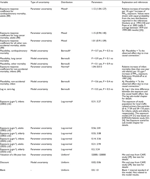
The effect of uncertainty was studied by conducting a comprehensive sensitivity analysis of a life-table model. Both parameter and model uncertainties were propagated through the model by Monte Carlo simulation. The model uncertainty was described with binary variables (Bernoulli distribution), choosing between two alterna-tive model branches (exception discount rate). Parameter uncertainty was described by using continuous distribu-tions. The effects of parameter and model uncertainties on model results were studied using sensitivity analysis. The sensitivity analysis was done by calculating absolute rank-order correlations between the input variables and the model results. All the studied input variables are pre-sented in table 1.
Life-expectancy (LE) and monetary value of lost life years were predicted. The LE was predicted by defining the change in the background hazard rate caused by local-traf-fic-related primary fine particles. The effects of fine parti-cles were predicted for both infants and adults. The time difference between an exposure and the consequent health effects (lag) was included in the model. The relative risk and lag estimates are described below. The monetary value of life-year-lost was predicted by calculating a value for a life year and discounting the future benefits and costs. The model was implemented using Analytica ™ ver-sion 3.1.1. (Lumina Deciver-sion Systems, Inc., CA) Monte Carlo simulation program and run with 5 000 iterations.
Exposure scenarios sub-model (∆Ek)
Table 1: Input variables included in the sensitivity analysis.
Variable Type of uncertainty Distribution Parameters Explanation and references
Exposure-response coefficient for
cardiopulmonary mortality, adults (RR)
Parameter uncertainty Mixeda 1.12 (1.04;1.27) Relative increase of mortality
per 10 µgm-3 increase of PM2.5 exposure. Values were drawn with equal probability from the two distributions reported in the references Dockery et al. 1993 [10] and Pope et al. 2002 (table 3, average between 1979 and 1999-200 results) [25]. Exposure-response
coefficient for lung cancer mortality, adults (RR)
Parameter uncertainty Mixed 1.15 (0.94;1.40)
Exposure-response coefficient for all other non-accidental mortality, adults (RR)
Parameter uncertainty Mixed 1.01 (0.91;1.09)
Plausibility, cardiopulmonary mortality
Model uncertainty Bernoullib P = 0.7 yes, P = 0.3 no AJc. Plausibility = "Is the observed effect due to true causal connection." Plausibility, lung cancer
mortality Model uncertainty Bernoulli P = 0.9 yes, P = 0.1 no
Plausibility, other mortality Model uncertainty Bernoulli P = 0.1 yes, P = 0.9 no Exposure-response
coefficient for non-accidental mortality, infants (RR)
Parameter uncertainty Normald 1.04; 0.013 Relative increase of infant
mortality (less than one year old infants) per 10 µgm-3 increase of PM2.5 exposure. Reference Woodruff et al. 1997 [30].
Plausibility, non-accidental
mortality, infant Model uncertainty Bernoulli P = 0.6 yes, P = 0.4 no AJ. Plausibility = "Is the observed effect due to true causal connection."
Lag vs. zero-lag Model uncertainty Bernoulli P = 0.5 yes, P = 0.5 no AJ. Lag = the time difference
between the exposure and the causal health effect. See The lag sub-model chapter for details.
Exposure (µgm-3), infants (2002) (∆E)
Parameter uncertainty Log-normale 0.31; 3.27 The exposure of study
population for local traffic related primary fine particles (0–6, 7–59 and 59–110 years for infants, adults and elderly, respectively). The exposure model [19–21] was based on EXPOLIS-Helsinki study [22– 24]. See Exposure scenarios sub-model chapter for details.
Exposure (µgm-3), adults (2002) (∆E)
Parameter uncertainty Log-normal 0.56; 2.81
Exposure (µgm-3), elderly (2002) (∆E)
Parameter uncertainty Log-normal 0.55; 3.08
Exposure (µgm-3), infants
(2025) (∆E) Parameter uncertainty Log-normal 0.14; 3.56
Exposure (µgm-3), adults
(2025) (∆E) Parameter uncertainty Log-normal 0.21; 2.94
Exposure (µgm-3), elderly
(2025) (∆E) Parameter uncertainty Log-normal 0.2; 3.24
Valuation of a life-year-lost Parameter uncertainty Uniformf 52000; 120000 Min and max from CAFE
study [39]. See text for details.
Discount Model uncertainty Uniform 0.02; 0.06 Min and max from CAFE
study [39]. See text for details.
Blank - Uniform 0.0; 1.0 Blank = internal standard of
the model. Not related to the model results.
a Mixed: Combination of two normally distributed variables (mean and 90% confidence intervals). b Bernoulli (binomial) binary probability distribution with probabilities (P, 1-P)
c AJ = Author judgment.
d Parameters for normal distribution (mean; standard deviation)
Health Effects caused by Urban Air Pollution for the Transport System Plan Scenarios in Helsinki Area (HEAT). The HEAT project evaluated traffic flows, air pollution emissions from traffic, resulting ambient air concentrations and exposures, and health effects in the Helsinki metropolitan area. The evaluations were done for two years, 2002 (cur-rent) and 2025 (the target year of the current transport system plan of this area). The traffic volumes for 2025 were assessed by combining Helsinki metropolitan area land use scenarios with a traffic demand model prepared by the Helsinki Metropolitan Area Council (YTV). The spatial distribution and the amount of key air pollution emissions, including fine particles, were predicted from the traffic flow estimations.
The hourly fine particle concentrations from primary traf-fic emissions over the Helsinki metropolitan area were computed by Finnish Meteorological Institute [16] within spatial resolution ranging from 10 to 500 meters. Ambi-ent concAmbi-entrations from local traffic were sampled for res-idential and occupational locations using a stratified random sampling scheme and small-area planning dis-tricts. Indoor concentrations of local traffic related fine particles were modelled using an infiltration model [17]. Concentrations experienced while in traffic were pre-dicted from EXPOLIS data [18] and scaled for the years 2002 and 2025 using predicted changes in tailpipe emis-sions. Population exposures were estimated separately for infants, adults, and elderly (0–1, 25–59, and 60–110 years, respectively). The exposure model [19-21] was based on EXPOLIS-Helsinki study [22-24] that measured exposure of adult population to various air pollutants in the study area. Exposures of the infants and the elderly were obtained by combining time activity data with the measured concentration data in relevant microenviron-ments. In the life-table model, the infant exposure was extended for years 0–6 (below school age) and adult expo-sure for the years 7–59 (table 1).
The exposure distributions were designed to represent individual variations in the personal exposures. These tributions are likely to be wider than the uncertainty dis-tributions for the age group averages, and therefore they provide an upper limit estimate of the importance of exposure uncertainty.
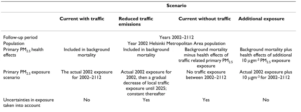
Four exposure scenarios (i-iv) were defined. (i) 'Current with traffic' scenario assumed that the exposure to local traffic related fine particles would remain at the year 2002 level. This is the base scenario used, and exposure uncer-tainties were not included for this scenario. This is because the combined effect of fine particle exposure and all other causes of mortality are seen in the current mortality statis-tics with very high precision and because the main aim is to focus on uncertainties related to fine particles.
There-fore, the uncertainties in the current exposure to fine par-ticle are propagated into scenarios ii and iii, which are expressed in comparison to the baseline scenario.
(ii) 'Reduced traffic emissions' scenario assumed that the exposure to fine particles due to local traffic would decline linearly between the years 2002 and 2025 and would remain constant thereafter. (iii) 'Current without traffic' scenario assumed that the exposure to all local-traffic-related fine particles was zero. Thus, the 'Current without traffic' scenario can be used to predict loss of life-expect-ancy due to traffic-related primary fine particles. (iv) The 'Additional exposure' scenario assumed a constant 10 µgm-3 exposure above the actual 2002 level after the year 2002 to the total population. The 'additional exposure' scenario was used to compare the magnitude of the health effects to those obtained in the other studies. The expo-sure scenarios and their properties are summarized in table 2.
Exposure-response sub-model (βobs)
An exposure-response model was built to describe the slope of the exposure-response function (βobs) of the PM2.5 health effects in adults and in infants. Multiple health outcomes have been detected in epidemiological studies in relation to PM2.5, but in this study we consid-ered only mortality due to long-term exposure. Slopes of the exposure-response functions were estimated based on the epidemiological studies conducted in the U.S [10,25]. Also the plausibility of association was included in the model, defined as the probability that the observed expo-sure-response association actually represents a causal association (table 1). The plausibility of a health effect was included in the exposure-response model using author judgment based on a previous work [5]. Both plau-sibility and exposure-response coefficient estimates and assumptions are presented in Table 1.
particles and total mortality, even though they used PM10 as a surrogate for particulate air pollution. The plausibility that the observed exposure-response association actually represents a causal association of the effect was assumed to be 60% (table 1).
The slope of the exposure-response function for the ages 1–110 was estimated based on epidemiological studies. There are several large epidemiological studies related to adult chronic PM2.5 exposure (e.g. [10,31-33]). We calcu-lated the concentration-response coefficient by drawing values with equal probability from the result distributions reported in the Dockery et al. 1993 and Pope et al. 2002 studies (table 1) [10,25]. These two studies were selected because they had focused on overall fine particles expo-sure (thus, not an any specific source), they meaexpo-sured all the relevant health outcomes, and because we assume them to be representative for primary fine particles present the Helsinki Metropolitan Area. The equal proba-bility was selected because we did not want to preferen-tially emphasize either one of these studies. The plausibility of the causal association for adult mortality was assumed separately for three mortality outcomes. We assumed that the probability for PM2.5 being the true cause of the effects is 70%, 90% and 10% for cardiopul-monary, lung cancer, and all other mortality, respectively. The plausibility for cancer was highest because there are known carcinogens in PM2.5 [34], while it is more debata-ble what agent is responsidebata-ble for the cardiovascular effects in the air pollution mix.
The lag sub-model (L)
Lag was defined as the time for how long a given fine par-ticle exposure (on a yearly basis) increases the incidence of a health effect. The effect, when measured as relative
risk, was assumed to be distributed evenly between expo-sure and the end of the lag period (see equation 1). The lag assumptions were based on the environmental tobacco smoke studies [35-38] and author judgment. For the lung cancer, cardiopulmonary, and all other non-acci-dental mortality, the lag was assumed to be 40, 15 and 1 years, respectively. The high lag assumptions were used to avoid any underestimation of the importance of this vari-able.
Monetary valuation
The monetary value of the years-of-life-lost and the rela-tive importance of the uncertainties related to monetary valuation were predicted to compare the relative impor-tance of the monetary valuation on the health effect uncertainties. The monetary valuation was based on the value for a life-year lost (VOLY) estimates and discount rates that were both adopted from The Clean Air for Europe (CAFE) program.
The value of a life-year lost estimate was based on CAFE program mean and median values (52000 and 120000 euros, respectively) [39]. The CAFE values were based mainly on the NewExt study [40]. That study developed an improved methodology for undertaking a monetary valuation of mortality impacts from air pollution by using the value-of-life-year-lost approach. We adopted the val-ues used in the CAFE program and expressed the uncer-tainty between the numbers with a uniform distribution (table 1).
Benefits from reduced fine particle exposure occur in the future. Discounting has been used in some fine particle health effect studies [13,14] to express the present values of these future benefits. The logic for this is that the
bene-Table 2: The description of different scenarios. See Exposure scenarios sub-model -chapter for details.
Scenario
Current with traffic Reduced traffic emissions
Current without traffic Additional exposure
Follow-up period Years 2002–2112
Population Year 2002 Helsinki Metropolitan Area population
Primary PM2.5 health
effects
Included in background mortality
Included in background mortality
Background mortality minus health effects of traffic related primary PM2.5
exposure
Background mortality plus health effects of additional
10 µgm-3 PM
2.5 exposure
Primary PM2.5 exposure
scenario
The actual 2002 exposure for 2002–2112
Actual 2002 exposure for 2002, then a gradual decrease of local traffic
exposure until 2025; constant thereafter
No traffic exposure between 2002–2112
Actual 2002 exposure plus 10 µgm-3 for 2002–2112
Uncertainties in exposure taken into account
fits are assumed to have lower utility, if they are post-poned into the distant future. Also the public seems to discount future benefits [41]. In the CAFE program 4% discount rate with 2% and 6% low and high estimates were used [39]. We adopted these numbers and expressed discount with uniform distribution ranging from 2% to 6% (table 1). Discounting was used only in monetary val-uation.
Background hazard rates (Hb)
The background hazard rates (Hb) for cardiopulmonary, lung cancer, other non-accidental, and accidental mortal-ity were defined as the average mortalmortal-ity occurring over the years 1988–2002 [42] (see additional file 1: Study population.pdf for the population and mortality data). Both mortality and population data were obtained for ages 0–99. The hazard rates of the oldest age group (95– 99) were used for the years 100–110. Mortality statistics had been coded using International Classification of Dis-ease (ICD) codes version 9 (years 1988–1995) and 10 (years 1996–2002). ICD codes for cardiopulmonary, lung cancer, and accidental mortality were 390–459, 1622– 1629, and 800–990, in version 9, respectively, and I00-I99, F01, and V01-Y89 in version 10. Four fifths of mortal-ity for the first age group (0-4-year-old) was assumed to occur during the first year of life.
Impact indicators
Life-expectancy (LE) indicator was predicted in the life-table model. The analyses were conducted for the Helsinki metropolitan area population (year 2002) of approx. 1 million inhabitants. The population age structure, includ-ing years lived before 2002, were taken into account in the life-expectancy indicator. The population was sub-divided into one-year age groups. The study population was fol-lowed until the age of 110 years.
The effect of PM exposure on mortality rate (m) ratio is typically predicted based on the following regression for-mula:
ln(m) = α+ β× E + ε (1)
where αis the background mortality coefficient, βis the exposure-response coefficient and E is exposure (εis a nui-sance parameter). Since we are interested in the effects of lag, we must assume that the observed βis actually a prod-uct effect resulting from a cumulative exposure that occurred before the observation. Thus,
where l is the time (in years) before the observation and Hb is the background hazard rate (see additional file 1:
Study population.pdf for the population and mortality data).
In this article we assume that the effects of a given expo-sure are evenly distributed in time between the expoexpo-sure and the lag L (after which no effects occur), and that in the cohort studies, the exposure was constant for at least L years. In such a scenario, we can see that:
where RRobs is the observed risk ratio per unit exposure of the exposure response function, and L is the maximum lag in years. The mortality rates (m) were estimated for each age group (ages 0–110) (i), year (years 2002–2112) (y), mortality outcome (four different outcomes) (j) and exposure scenarios (scenarios i-iv) (k). The calculated mortality rates were then used to predict the survival of the year 2002 population in the future.
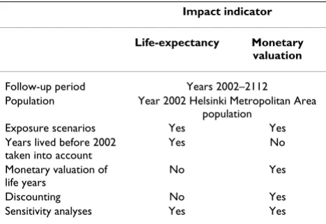
The life-expectancy was predicted for the study popula-tion by summing the years lived before 2002 and years lived during the study time (years 2002–2112) and divid-ing the sum with the year 2002 population size. The mon-etary valuation was based on years-of-life-lost which differed from the LE method by considering only the years to be lived during the follow-up period and by estimating the effects of fine particle exposure using monetary indica-tor (euros). The differences between life-expectancy and monetary valuation impact indicators are summarized in table 3. See additional file 2 for the complete model.
Results
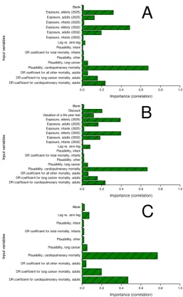
Factors identified as highly important included both parameter and model uncertainties (Figure 1A–1C). The plausibility of cardiopulmonary mortality (model uncer-tainty) exhibited the highest importance in all scenarios. The exposure-response coefficient of cardiopulmonary mortality (parameter uncertainty) displayed high
impor-m= + lL ×El =Hb× lL ×El
= =
∑
∑
exp(α 0(β )) exp( 0(β ))
(2)
exp( )β =LRRobs (3)
Table 3: The main properties of two impact indicators.
Impact indicator
Life-expectancy Monetary valuation
Follow-up period Years 2002–2112
Population Year 2002 Helsinki Metropolitan Area population
Exposure scenarios Yes Yes
Years lived before 2002 taken into account
Yes No
Monetary valuation of life years
No Yes
Discounting No Yes
Results from sensitivity analyses of the input variables Figure 1
Results from sensitivity analyses of the input variables. The bars show how each individual input variable correlated with the model output. The high correlations indicate that the input variable has a strong impact on the model output. The results are relative, such that removal of one uncertainty will affect the sensitivity of the other uncertainties. Sensitivity analysis was done by calculating absolute rank-order correlations between the input variables and the model output. A. Impact indica-tor life-expectancy using the 'Current without traffic' scenario. B. Impact indicaindica-tor monetary valuation using the difference between 'Current without traffic' and 'Reduced traffic emissions' scenarios. C. Impact indicator life-expectancy using the 'Addi-tional exposure' scenario. ER = exposure-response.
DR coefficient for cardiopulmonary mortality, adults DR coefficient for lung cancer mortality, adults DR coefficient for all other mortality, adults Plausibility, cardiopulmanary mortality Plausibility, lung cancer Plausibility, other DR coefficient for total mortality, infants Plausibility, infant Lag vs. zero-lag Blank
0.0 0.2 0.4 0.6 0.8 1.0
A
Importance (correlation)
In
p
u
t v
a
ri
a
b
le
s
DR coefficient for cardiopulmonary mortality, adults DR coefficient for lung cancer mortality, adults DR coefficient for all other mortality, adults Plausibility, cardiopulmanary mortality Plausibility, lung cancer Plausibility, other DR coefficient for total mortality, infants Plausibility, infant Lag vs. zero-lag Exposure, infants (2002) Exposure, adults (2002) Exposure, elderly (2002) Exposure, infants (2025) Exposure, adults (2025) Exposure, elderly (2025) Valuation of a life-year-lost Discount Blank
0.0 0.2 0.4 0.6 0.8 1.0
B
Importance (correlation)
In
p
u
t v
a
ri
a
b
le
s
DR coefficient for cardiopulmonary mortality, adults DR coefficient for lung cancer mortality, adults DR coefficient for all other mortality, adults Plausibility, cardiopulmanary mortality Plausibility, lung cancer Plausibility, other DR coefficient for total mortality, infants Plausibility, infant Lag vs. zero-lag Exposure, infants (2002) Exposure, adults (2002) Exposure, elderly (2002) Exposure, infants (2025) Exposure, adults (2025) Exposure, elderly (2025) Blank
0.0 0.2 0.4 0.6 0.8 1.0
C
Importance (correlation)In
p
u
t v
a
ri
a
b
le
tance. Uncertainties related to lung cancer mortality and other, non-accidental, mortality had low or negligible importance. The results of the sensitivity analyses were as expected because of the high background mortality rates for cardiopulmonary mortality. The results of the sensitiv-ity analyses were double-checked with a modified value-of-information analysis [2], in which the model result was tested against the expectation value of the model. The benefit of value of information analysis is that it is a deci-sion analysis method that estimates the benefits of collect-ing additional information and expresscollect-ing it in a common metric. Thus, it can be used to evaluate the importance of a particular input variable (as in this case). The value of information analysis confirmed the sensitivity analyses results (data not shown). These results highlight the importance of the cardiopulmonary mortality in compar-ison to the other mortality outcomes.
The plausibility and exposure-response coefficients related to infant mortality had minor importance in all sensitivity analyses (figure 1A–1C). Thus, infant mortality makes a low contribution to the population life-expect-ancy although the individual loss of life is considerable. However, the results would be expected to be different in developing countries due to differences in the background infant mortality rates and different cause-specific rates.
The lag vs. zero-lag input variable (model uncertainty) seemed to be of minor importance (figure 1A–C). The a priori hypothesis was that lag could be important since the Finnish population is relatively old on average, and a long lag could prevent the impact of lowering exposures from benefiting for elderly subjects. It should be noted that the lag assumptions used in this study were exceed-ingly long, although a few intervention studies, especially
the coal ban in Dublin [31] and the Utah valley steel mill strike [43], suggest that the major part of the effect is seen within the first few years.
Discount and value of life-year-lost variables were very important in comparison to the life-expectancy uncertain-ties (figure 1B). The results showed how the uncertainuncertain-ties related to placing a monetary valuation on the effects of air pollution could have a more significant impact on the results of the model than many input variables connected to health effects evaluation. The effect of discount for the different age groups is presented in Figure 2, showing clearly how high discounts reduce the benefit to the younger age groups if compared with those over 60 years. On the other hand, the discounting did not affect the ben-efits to people over 80 years of age.
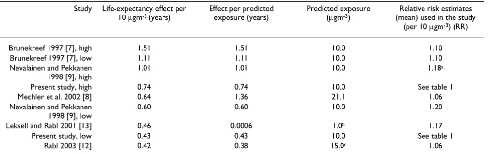
The continued exposure to 10 µgm-3 fine particles lowered the life-expectancy of the study population by 0.41 years (mean; 90% confidence interval: 0.00 – 1.04). Previous life-table models have predicted that the continued expo-sure to 10 µgm-3 fine particles would lowers the life-expectancy by anything between 0.42–1.5 years (table 4). The magnitude of life-expectancy loss was lower in the present study than in some of the previous life-table mod-els. However, when the present model was run with a birth cohort of imaginary 100000 children, without plau-sibility estimations, and with the years 1988–1990 back-ground hazard rates, the life-expectancy loss was 0.74 (mean, 90% CI 0.23 – 1.44) years (with 10 µgm-3 PM
2.5 exposure). Even though the model uncertainties had sig-nificant effects on model results, they were in agreement with previous models results.
Table 4: Comparison of the results of different life-table studies.
Study Life-expectancy effect per 10 µgm-3 (years)
Effect per predicted exposure (years)
Predicted exposure (µgm-3)
Relative risk estimates (mean) used in the study
(per 10 µgm-3) (RR)
Brunekreef 1997 [7], high 1.51 1.51 10.0 1.10
Brunekreef 1997 [7], low 1.11 1.11 10.0 1.10
Nevalainen and Pekkanen 1998 [9], high
1.01 1.01 10.0 1.18a
Present study, high 0.74 0.74 10.0 See table 1
Mechler et al. 2002 [8] 0.64 1.36 21.1 1.06
Nevalainen and Pekkanen 1998 [9], low
0.60 0.60 10.0 1.20
Leksell and Rabl 2001 [13] 0.46 0.0006 1.0b 1.17
Present study, low 0.43 0.43 10.0 See table 1
Rabl 2003 [12] 0.42 0.38 15.0c 1.06
The results have been scaled to 10 µgm-3 PM
2.5 exposure by assuming log-linearity between increased particle exposure and loss in life-expectancy.
The exposure of the elderly is the most important uncer-tainty of all the exposure variables (figure 1A–1B). This seems logical, as most of the health effects have been observed in the older age groups. The use of individual variation in exposure assessment overestimated the uncer-tainty of the average population exposure and could therefore lower the importance of other input variables. However, when additional analyses were conducted with-out exposure variability, it was noted that exposure did not significantly affect the importance of the other input variables (data not shown).
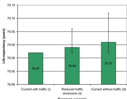
The life-expectancy predictions for the three exposure sce-narios are presented in Figure 3. The difference between the 'Current with traffic' and 'Current without traffic' sce-narios was 0.04 years (mean, 90% CI -0.15 – 0.00), repre-senting the life-expectancy loss in the study population due to local traffic-related primary fine particles. In abso-lute numbers (premature death) the local traffic was pre-dicted to be responsible for 3.7, 27.2, and 0.2 lung cancer, cardiopulmonary and other non-accidental mortality out-comes in the year 2002, respectively. In the monetary val-uation, the difference between the scenarios was 880 million euros/million inhabitants (when taking into account discount and the monetary values from the year 2002 onward). The decline in fine particles exposure by 2025, as predicted here based on the HEAT -project, improves the expected life-expectancy by 0.02 years. In the monetary valuation, the benefits were predicted to be 390 million euros/million inhabitants (from year 2002
onward). These benefits materialize in the year 2002 cohort that was followed until the year 2112. The benefits for the society are larger because the benefits to other peo-ple in the future population are not included. The local traffic-generated primary fine particles were shown to have a significant effect on health status of the study pop-ulation.
Discussion
In this study, we have made a comprehensive sensitivity analysis of a fine particle life-table model. The uncertain-ties relating to cardiopulmonary mortality have large effects on life-table model results, whereas the uncertain-ties attributable to lag and infant mortality have only minor effects. The discount and value of a life-year varia-bles had significant impact on the results when estimating the monetary loss of the life years. The variability of expo-sure had major effects on the life-table model results. These results provided valuable information on the rela-tive importance of different input variables in the life-table model and make it possible to focus on those varia-bles and uncertainties that have the highest impact on to life-table model results and, thus, on decision making.
The sensitivity analyses showed that the life-table model result is mainly attributable to the contribution of
cardi-Life-expectancy predictions for three different exposure sce-narios
Figure 3
Life-expectancy predictions for three different expo-sure scenarios. Predicted life-expectancy for three differ-ent exposure scenarios (mean and 90% confidence intervals shown). The difference between scenarios 'Current without traffic' and 'Current with traffic' represents the current life-expectancy loss in Helsinki Metropolitan Area due to local traffic emitted primary fine particles emissions. The 'Reduced traffic emissions' scenario describes the effect of a plausible emission reduction scenario for 2002–2025.
78.97 78.99
79.01
78.85 78.90 78.95 79.00 79.05 79.10 79.15
Current with traffic (i) Reduced traffic emissions (ii)
Current without traf
Exposure scenario
L
if
e-exp
ect
an
cy (
year
s)
fic (iii)
Life-years-lost costs due to fine particle exposure with differ-ent discount rates
Figure 2
Life-years-lost costs due to fine particle exposure with differ-ent discount rates.
0 20 40 60 80 100
0 200 400 600 800 1000 1200 1400 1600
Loss per person
(eu
ros)
Age in year 2002
opulmonary mortality. This was expected since the back-ground cardiopulmonary mortality is higher than lung cancer or non-accidental mortality and changes (and uncertainties) related to the concentration-response func-tion of cardiopulmonary mortality was expected to have a major effect on the results. There are no significant differ-ences in the magnitude of the effect between studies that have separated the mortality outcomes (present study and Nevalainen and Pekkanen study [9]) and studies that have not (all others in table 4). Cardiopulmonary mortality is declining in the developed countries, and this may affect the results from fine particle life-table models if different mortality outcomes are not separated in the analyses.
The plausibility was defined in this study as the probabil-ity that the observed exposure-response association actu-ally represents a causal association. The separation of causal relationship and the exposure-response function have also been under examination in the recent expert elicitation study prepared by U.S. EPA [44]. The experts were asked to give their best estimate for the likelihood that there is a causal relationship between fine particles and all-cause mortality. Their answers ranged from 100% to 35%, though the majority of the experts thought that the likelihood would be 95% or more [44]. In addition to their best judgment, the expert also provided an estimate of range. Our approach differs from the EPA study, so that we separated the different mortality outcomes and used only the best estimates. As an alternative approach, we could also have tested the uncertainty around our best guess for plausibility. However, it could also be argued that plausibility is an inherently dichotomous variable and the truth is always either zero or one.
When analyzing the importance of plausibility, we used low plausibility estimates for different mortality out-comes. It could be argued that this would overestimate the current uncertainty on the plausibility of the association between fine particles, especially for lung cancer, but probably also for cardiovascular disease. With respect to lung cancer, few experts have challenged the plausibility for an association, but even for cardiovascular disease there is more and more evidence to support the existence of plausible mechanisms for an association [34,44,45]. However, the value 35%, represented in [44], shows that the plausibility is still a major issue, although the current evidence had convinces most of the experts [44]. The plausibility assumptions have been estimated in our pre-vious study [5] and the true uncertainty based on current knowledge would probably show higher plausibility and thus have lower importance in this analysis.
In the present study, various causes of death were assumed to be statistically unrelated. The assumption means that the individuals who benefit from lowering risks (by
removing the underlying cause of death) have a similar probability to survive as the individuals that were not threatened by the risk in the first place (in other words, people who benefit do not have more competing causes than the general population). It is likely that this assump-tion is not completely valid as such. Mackenbach et al. have investigated this question in a number of statistical studies by comparing the magnitude of competing causes in different underlying mortality outcomes from the Dutch national cause-of-death register [46-48]. In their latest analyses, they concluded that the prevalence of the competing causes is high with respect to respiratory dis-eases, about average with cardiovascular disdis-eases, and low with neoplasms [48]. This implies that patients with a neoplasm have a lower risk of dying of other causes if they survive the neoplasm. If applicable to this analysis, these results could mean that the present life-table model may over-predict the import of the cardiopulmonary mortality while underestimating the import of the lung cancer.
The results from sensitivity analyses showed that both dis-count rate and value of year had a large impact on life-table model results when the results are presented using monetary indicators. The monetary valuation was also noted to be a major source of uncertainty in the CAFE uncertainty analyses, when taking into account the full chain of cost-benefit analysis [15]. The use of a monetary valuation and discount in the health risk assessment is a controversial issue. The driving force behind our analysis was to compare the uncertainties related to health effect variables with the corresponding uncertainties in mone-tary variables. Our intention was not to commit on discus-sion whether or not health effect should be valued in monetary terms. The results suggested that uncertainties related to monetary valuation are at least as important for the results as the most important health evaluation varia-bles.
younger age groups and relatively emphasizes effects for the middle-aged population (50 to 70 years old).
The lag has been used in some previous life-table studies. Leksell and Rabl [13] used a repair model to calculate the decline in the relative risk (repair process) after a decline in the exposure to fine particles. That model was based on the time constant, which they measured from tobacco smoking studies. Röösli et al. [50] adopted the Leksell and Rabl model, but they used air pollution intervention stud-ies to calculate a time constant. Both models measured the association between fine particles and total non-acciden-tal mornon-acciden-tality. Although the authors estimated time con-stants based on different studies, they both concluded that it had little or no effect on life-table model results [13,50]. A similar result was seen in this study, although both the lag sub-model and the lag assumptions used were differ than those in the previous studies. The lag sub-model used in this study assumed that the adverse effect of fine particles would grow gradually while other models have used delay functions. Therefore, the results of the present study and the results from these other life-table models are not fully comparable. However, taken together, it could be concluded that lag is not an important input var-iable for the fine particle life-table models and therefore it could be ignored in future analyses.
Local traffic-related fine particles were shown to have a notable effect on study population. However, this was only a small part of the total exposure as the difference between PM2.5 exposure scenarios were about or less than 0.5 µgm-3 while the total exposure in the study area is about 10 µgm-3 [24]. The health effects of local traffic-related particles were also addressed only for the local population and thus the total health effects would have been larger had the dispersion of pollutants outside the study area been taken into account. Three of four exposure scenarios were based on the HEAT-project that evaluated traffic flows, air pollution emissions from traffic, resulting ambient air concentrations and exposures, and health effects in the study area. The scenarios took account of the land use policy, changes in traffic flows and emissions and the location and the time activity of the population. The comparison of the exposure scenarios showed that with the current policy, about half of the primary fine particles effects due to local traffic can be avoided within twenty years. The results show that the current actions are head-ing in the right direction. However, more rapid actions could be implemented, as the current transport system plan is mostly focussed on road construction and public transport subsidies and less on emission control, traffic demand, or prevention of infiltration of outdoor particles into buildings [51].
Conclusion
The uncertainties of a life-table model for estimation of population health risks caused by local primary traffic particles were investigated in detail using a sensitivity analysis approach. The main results were: (i) uncertainties in several input variables as well as in the model structure were noted to have large effects on the model results. (ii) The uncertainty in the plausibility of the cardiopulmonary mortality, the exposure-response coefficient for cardiopul-monary mortality, and PM2.5 exposure in the elderly pop-ulation were major sources of uncertainty, whereas (iii) uncertainty in the variables lag vs. zero-lag, exposure-response coefficient for total mortality of infants, plausi-bility of infant mortality effects, and other non-accidental mortality were not major sources of uncertainty. The dis-count and value of a life-year variables did have a signifi-cant impact on the results when comparing the results of two different exposure scenarios. The estimates used for cardiopulmonary PM coefficient, plausibility, and PM2.5 exposure warrant updated estimates based on the current scientific evidence. The discount rate is more of a political issue, but this analysis showed that it is important to be explicit about this issue. In contrast, complicated lag struc-tures can be omitted without this having any major impact on the results. The fine particle emissions attribut-able to local traffic were shown to cause significant life-expectancy loss in the Helsinki metropolitan area popula-tion.
Abbreviations
AJ- Author judgmentCAFE- Clean Air for Europe program
CI- Confidence interval
EPA- U.S. Environmental Protection Agency
ER- Exposure-response
EXPOLIS- Air Pollution Exposure Distributions of Adult Urban Populations in Europe -study
Hb- The background hazard rate of the study population
HEAT- Health Effects caused by Urban Air Pollution for the Transport System Plan Scenarios in Helsinki Area -study
ICD- International Classification of Disease -code
LE- Life-expectancy
PM10- Thoracic particulate matter (particles with aerody-namic diameter less than 10 micrometers)
PM2.5- Fine particulate matter (particles with aerodynamic diameter less than 2.5 micrometers)
RR- Relative risk
TSP- Total suspended particles
VOLY- Valuation of a life-year-lost
YOLL- Years-of-life-lost
YTV- Helsinki Metropolitan Area Council
Competing interests
The author(s) declare that they have no competing inter-ests.
Authors' contributions
MT conceived the study, performed modeling and drafted the manuscript. JTT and OH participated in the design of the study, helped with the modeling and with the manu-script drafting. OH ran the exposure models. JR, MJJ and JP participated in the design of the study and helped with the manuscript drafting. All authors have read and approved the final manuscript.
Additional material
Acknowledgements
This study was conducted in the National Public Health Institute, Centre for Environmental Health Risk Analysis; and in the University of Kuopio. The Centre was funded by the Academy of Finland (Grant 53307) and the National Technology Agency of Finland (Tekes) (Grant 40715/01). This study was done as a part of the projects HEAT (funded by the Academy of Finland, Grant 53246), KOPRA (funded by the Ministry of the Environment,
Finland, Grant YM119/481/2002, the National Technology Agency of Fin-land (Tekes), Grant 616/31/02 and the Helsinki Metropolitan Area Council (YTV), Grant 135/03), PILTTI (funded by the Ministry of the Environment, Finland, Grant YM57/065/2005), INTARESE (funded by European Union, Grant 018385-2) and SCUD (funded by the Academy of Finland, Grant 111775).
We would like to thank Mr. Pekka Tiittanen for providing and management of the mortality data. We would also like to thank Dr. Ewen MacDonald for checking the English language.
References
1. Linkov I, Burmistrov D: Model uncertainty and choices made by modelers: Lessons learned from the international atomic energy agency model intercomparisons. Risk Anal 2003,
23(6):1297-1308.
2. Morgan MG, Henrion M: Uncertainty a guide to dealing with uncertainty in quantitative risk and policy analysis. Cam-bridge , CamCam-bridge University Press; 1990:xii, 332 s..
3. Watkiss P, Steve P, Mike H: Baseline scenarios for service con-tract for carrying out cost-benefit analysis of air quality related issues, in particular in the clean air for Europe (CAFE) programme. Didcot, UK , AEA Technology Environment; 2005.
4. Forsberg B, Hansson HC, Johansson C, Areskoug H, Persson K, Järvholm B: Comparative health impact assessment of local and regional particulate air pollutants in Scandinavia. Ambio 2005, 34(1):11-19.
5. Tainio M, Tuomisto JT, Hanninen O, Aarnio P, Koistinen KJ, Jantunen MJ, Pekkanen J: Health effects caused by primary fine particu-late matter (PM2.5) emitted from buses in the Helsinki met-ropolitan area, Finland. Risk Anal 2005, 25(1):151-160. 6. Miller BG, Hurley JF: Life table methods for quantitative impact
assessments in chronic mortality. J Epidemiol Community Health 2003, 57(3):200-206.
7. Brunekreef B: Air pollution and life expectancy: is there a rela-tion? Occup Environ Med 1997, 54(11):781-784.
8. Mechler R, Amann M, Schöpp W: A methodology to estimate changes in statistical life expectancy due to the control of particulate matter air pollution. Laxenburg, Austria , Interna-tional Institute for Applied System Analysis (IIASA); 2002.
9. Nevalainen J, Pekkanen J: The effect of particulate air pollution on life expectancy. Sci Total Environ 1998, 217(1-2):137-141. 10. Dockery DW, Pope CA III, Xu X, Spengler JD, Ware JH, Fay ME,
Fer-ris BG Jr., Speizer et : An association between air pollution and mortality in six U.S. cities. N Engl J Med 1993,
329(24):1753-1759.
11. Pope CA, Thun MJ, Namboodiri MM, Dockery DW, Evans JS, Speizer FE, Heath CW: Particulate air-pollution as a predictor of mor-tality in a prospective-study of US adults. Am J Respir Crit Care Med 1995, 151(3):669-674.
12. Rabl A: Interpretation of air pollution mortality: Number of deaths or years of life lost? J Air Waste Manag Assoc 2003,
53(1):41-50.
13. Leksell I, Rabl A: Air pollution and mortality: Quantification and valuation of years of life lost. Risk Anal 2001, 21(5):843-857. 14. Coyle D, Stieb D, Burnett RT, DeCivita P, Krewski D, Chen Y, Thun MJ: Impact of particulate air pollution on quality-adjusted life expectancy in Canada. J Toxicol Environ Health 2003, 66(16-19):1847-1863.
15. Holland M, Hurley F, Hunt A, Watkiss P: Methodology Paper (Vol-ume 3) for Service Contract for carrying out cost-benefit analysis of air quality related issues, in particular in the clean air for Europe (CAFE) programme. Didcot, UK , AEA Technol-ogy Environment; 2005.
16. Kauhaniemi M, Karppinen A, Härkönen J, Kousa A, Koskentalo T, Aarnio P, Kukkonen J: Refinement And Statistical Evaluation Of A Modelling System For Predicting Fine Particle Concentra-tions In Urban Areas: 27-29 March; Limassol, Cyprur.
Edited by: Sokhi RS, Neophytou M. ; 2007.
17. Hanninen OO, Lebret E, Ilacqua V, Katsouyanni K, Kunzli F, Sram RJ, Jantunen M: Infiltration of ambient PM2.5 and levels of indoor generated non-ETS PM2.5 in residences of four European cities. Atmos Environ 2004, 38(37):6411-6423.
Additional file 1
Study population. Population, mortality and background hazard rate (Hb) statistics of the study population.
Click here for file
[http://www.biomedcentral.com/content/supplementary/1476-069X-6-24-S1.pdf]
Additional file 2
The life-table model. The model contains the full model including the code and the descriptions. ANA (Analytica™ 3.1.1. file in XML format). For a free Analytica browser, see http://www.lumina.com/. Model identifier (unified resource name) is URN:NBN:fi-fe20061261. For more instruc-tions, see http://www.ktl.fi/risk.
Click here for file
Publish with BioMed Central and every scientist can read your work free of charge
"BioMed Central will be the most significant development for disseminating the results of biomedical researc h in our lifetime."
Sir Paul Nurse, Cancer Research UK
Your research papers will be:
available free of charge to the entire biomedical community
peer reviewed and published immediately upon acceptance
cited in PubMed and archived on PubMed Central
yours — you keep the copyright
Submit your manuscript here:
http://www.biomedcentral.com/info/publishing_adv.asp
BioMedcentral
18. Jantunen M, Hänninen O, Ilacqua V, Karppinen A, Kukkonen J, Aarnio P: Exposure levels to exhaust-generated and total PM2.5 in traffic: 29-31 March; Valencia, Spain. Edited by: Sokhi RS, Mil-lán MM, Moussiopoulos N. ; 2005.
19. Hanninen O, Kruize H, Lebret E, Jantunen M: EXPOLIS simulation model: PM2.5 application and comparison with measure-ments in Helsinki. J Expo Anal Environ Epidemiol 2003, 13(1):74-85. 20. Kruize H, Hanninen O, Breugelmans O, Lebret E, Jantunen M:
Description and demonstration of the EXPOLIS simulation model: Two examples of modeling population exposure to particulate matter. J Expo Anal Environ Epidemiol 2003,
13(2):87-99.
21. Hanninen OO, Tuomisto JT, Jantunen MJ: Characterization of model error in a simulation of fine particulate matter expo-sure distributions of the working age population in Helsinki, Finland. J Air Waste Manag Assoc 2005, 55(4):446-457.
22. Jantunen MJ, Hanninen O, Katsouyanni K, Knoppel H, Kuenzli N, Leb-ret E, Maroni M, Saarela K, Sram R, Zmirou D: Air pollution expo-sure in European cities: The "EXPOLIS" study. J Expo Anal Environ Epidemiol 1998, 8(4):495-518.
23. Rotko T, Oglesby L, Kunzli N, Jantunen MJ: Population sampling in European air pollution exposure study, EXPOLIS: compari-sons between the cities and representativeness of the sam-ples. J Expo Anal Environ Epidemiol 2000, 10(4):355-364.
24. Koistinen KJ, Edwards RD, Mathys P, Ruuskanen J, Kunzli N, Jantunen MJ: Sources of fine particulate matter in personal exposures and residential indoor, residential outdoor and workplace microenvironments in the Helsinki phase of the EXPOLIS study. Scandinavian Journal of Work Environment & Health 2004, 30, suppl 2:36-46.
25. Pope CA III, Burnett RT, Thun MJ, Calle EE, Krewski D, Ito K, Thurston GD: Lung cancer, cardiopulmonary mortality, and long-term exposure to fine particulate air pollution. JAMA:
The Journal Of The American Medical Association 2002,
287(9):1132-1141.
26. Sram RJ, Binkova BB, Dejmek J, Bobak M: Ambient air pollution and pregnancy outcomes: A review of the literature. Environ Health Perspect 2005, 113(4):375-382.
27. Glinianaia SV, Rankin J, Bell R, Pless-Mulloli T, Howel D: Does par-ticulate air pollution contribute to infant death? A system-atic review. Environ Health Perspect 2004, 112(14):1365-1371. 28. Tong SL, Colditz P: Air pollution and sudden infant death
syn-drome: a literature review. Paediatr Perinat Epidemiol 2004,
18(5):327-335.
29. McDonnell WF, Nishino-Ishikawa N, Petersen FF, Chen LH, Abbey DE: Relationships of mortality with the fine and coarse frac-tions of long-term ambient PM10 concentrafrac-tions in non-smokers. J Expo Anal Environ Epidemiol 2000, 10(5):427-436. 30. Woodruff TJ, Grillo J, Schoendorf KC: The relationship between
selected causes of postneonatal infant mortality and partic-ulate air pollution in the United States. Environ Health Perspect 1997, 105(6):608-612.
31. Clancy L, Goodman P, Sinclair H, Dockery DW: Effect of air-pollu-tion control on death rates in Dublin, Ireland: an interven-tion study. Lancet 2002, 360(9341):1210-1214.
32. Hoek G, Brunekreef B, Goldbohm S, Fischer P, van den Brandt PA:
Association between mortality and indicators of traffic-related air pollution in the Netherlands: a cohort study. Lan-cet 2002, 360(9341):1203-1209.
33. Pope CA, Burnett RT, Thurston GD, Thun MJ, Calle EE, Krewski D, Godleski JJ: Cardiovascular mortality and long-term exposure to particulate air pollution - Epidemiological evidence of general pathophysiological pathways of disease. Circulation 2004, 109(1):71-77.
34. Cohen AJ: Outdoor air pollution and lung cancer. Environ Health Perspect 2000, 108:743-750.
35. Doll R, Peto R, Boreham J, Sutherland I: Mortality in relation to smoking: 50 years' observations on male British doctors. Br Med J 2004, 328(7455):1519-1528.
36. Dockery DW, Trichopoulos D: Risk of lung cancer from envi-ronmental exposures to tobacco smoke. Cancer Causes Control 1997, 8(3):333-345.
37. Steenland K, Thun M, Lally C, Heath C: Environmental tobacco smoke and coronary heart disease in the American Cancer Society CPS-II cohort. Circulation 1996, 94(4):622-628.
38. Hackshaw AK, Law MR, Wald NJ: The accumulated evidence on lung cancer and environmental tobacco smoke. Br Med J 1997,
315(7114):980-988.
39. Hurley F, Hunt A, Cowie H, Holland M, Miller B, Pye S, Watkiss P:
Methodology Paper (Volume 2) for Service Contract for car-rying out cost-benefit analysis of air quality related issues, in particular in the clean air for Europe (CAFE) programme. In Methodology for the Cost-Benefit analysis for CAFE: Volume 2: Health Impact Assessment AEA Technology Environment; 2005.
40. IER: New Elements for the Assessment of External Costs from Energy Technologies. Institute for Energy Economics and the Rational Use of Energy (IER), University of Stuttgart; 2004. 41. Cropper ML, Aydede SK, Portney PR: Preferences for Life Saving
Programs - How the public discounts time and age. J Risk Uncertain 1994, 8(3):243-265.
42. Statistics Finland: Population and mortality data for year 1988-2002. Statistics Finland; 2005.
43. Pope CA, Schwartz J, Ransom MR: Daily Mortality and PM10 Pol-lution in Utah Valley. Arch Environ Health 1992, 47(3):211-217. 44. IEC, Industrial Economics: Expanded Expert Judgment
Assess-ment of the Concentration-Response Relationship Between PM2.5 Exposure and Mortality. Cambridge , Industrial Econom-ics; 2006.
45. Brook RD, Franklin B, Cascio W, Hong Y, Howard G, Lipsett M, Luepker R, Mittleman M, Samet J, Smith SC Jr., Tager I: Air pollution and cardiovascular disease: a statement for healthcare pro-fessionals from the Expert Panel on Population and Preven-tion Science of the American Heart AssociaPreven-tion. Circulation 2004, 109(21):2655-2671.
46. Mackenbach JP, Kunst AE, Lautenbach H, Bijlsma F, Oei YB: Com-peting causes of death - An analysis using multiple-cause-of-death data from the Netherlands. Am J Epidemiol 1995,
141(5):466-475.
47. Mackenbach JP, Kunst AE, Lautenbach H, Oei YB, Bijlsma F: Com-peting causes of death: A death certificate study. J Clin Epide-miol 1997, 50(10):1069-1077.
48. Mackenbach JP, Kunst AE, Lautenbach H, Oei YB, Bijlsma F: Gains in life expectancy after elimination of major causes of death: revised estimates taking into account the effect of compet-ing causes. J Epidemiol Community Health 1999, 53(1):32-37. 49. Pandey MD, Nathwani JS: Canada wide standard for particulate
matter and ozone: Cost-benefit analysis using a life quality index. Risk Anal 2003, 23(1):55-67.
50. Röösli M, Künzli N, Braun-Fahrländer C, Egger M: Years of life lost attributable to air pollution in Switzerland: dynamic expo-sure-response model. Int J Epidemiol 2005, 34(5):1029-1035. 51. YTV: Helsinki Metropolitan Area transport system plan PLJ