Investigation of the Dynamic Performance of a Cable-Stayed Footbridge

(1)

University of Trento University of Brescia University of Padova University of Trieste University of Udine University IUAV of Venezia

Anil Kumar

INVESTIGATION OF THE DYNAMIC PERFORMANCE OF A

CABLE-STAYED FOOTBRIDGE

Tutor: Prof. Oreste S. Bursi

(2)

UNIVERSITY OF TRENTO

Structural Engineering - Modelling, Preservation and Control of Materials and Structures

Cycle: XXIII

Head of the Doctoral School: Prof. Davide Bigoni

Board of Examiners:

Prof. Maurizio Piazza (Università degli Studi di Trento)

(3)

SUMMARY

The developments in conceptual design, material technology and efficient construction

techniques enabled the creation of longer, lighter, slender and stylish Cable-Stayed Foot

Bridges (CSFB). Hence, modern CSFB can be characterized by interacting phenomena like

cable nonlinearities, deck dynamic instability and deck lateral oscillations due to pedestrian

walking. These phenomena, if intertwined, may bring these structures out of service or to failure.

In view of a better performance, additional damping can be provided by passive dampers.

However, amplitude dependent behaviour of dampers and slip in connections can make them

effective only above a threshold amplitude. Hence, due to high uncertainties in the complex

CSFB-damper system, usually, dynamic tests are performed to investigate the performance of

the overall system.

In this thesis, the effectiveness of the passive vibration reduction system in a complex

cable-stayed footbridge characterised by two curved decks was investigated. The amplitude

dependent behaviour was found both with the output-only ambient vibration and free decay

tests. In order to clarify these outcomes, modal quantities were calculated instantaneously,

based on time-frequency identification techniques. A thorough analysis of dynamic response

signals revealed that the structure with dampers actually behaved like a threshold system: i) for

low vibration levels the dampers were still, so that they performed as constraints that stiffened

the structure; ii) for high vibration levels, the dampers became fully working. Moreover, a

deck-cable interaction between one of the longest deck-cables and the first global mode was detected.

Initially, the modal properties estimated from the dynamic tests did not match those of the

numerical model. In order to have a robust FE model capable to simulate the actual behaviour

of the footbridge, model updating was performed. The sensitivity-based model updating

techniques and Powell's Dog-Leg method of optimisation based on the Trust-Region approach

were used. The final updated model showed a considerable reduction in the percentage error of

frequencies. The updated model was able to reproduce the response of the footbridge under

actual wind conditions. The revealed cable-deck interaction phenomenon was a motivation to

investigate in depth the dynamics of long stay cables. Therefore, efforts were made towards the

identification of the nonlinear behaviour of stay cables from measured response data. In view of

the fact that actual measured data contained the response of a MDoF system, the first step in

this direction was to investigate the feasibility of the nonlinear identification method, i.e. a

non-parametric approach applied to a SDoF cable system. The results revealed a good fitting

between identified and numerical data, where only a cubic type of nonlinearity was identified.

Moreover, an increase of the parameter related to damping and a decrease of the parameter

relevant to linear-frequency were observed versus the loading amplitude. However, the values

of the parameters stabilised at higher load amplitudes and superharmonics were present in the

response. The proposed non-parametric method exhibited a good capability in the nonlinear

parameter identification of cables.

(4)

(5)

(6)

ACKNOWLEDGEMENTS

I would like to express my deepest gratitude and thanks to Professor Oreste S. Bursi for his

constant encouragement, guidance, kindness and his patience with me. I feel honoured to be

the student of Prof. Bursi.

Second, I would like to give my deep thanks to Dr. Silvano Erlicher (Ecole Nationale des Ponts

et Chaussees,-ENPC- France) and Dr. Rosario Ceravolo (Politecnico di Torino, Italy) for helping

me with their experiences and knowledge in the course of my research work. Here, I would like

to thank also to my colleagues Mr. Philippe Pecol from ENPC and Mr. Luca Zanotti Fragonara

from the Politecnico di Torino, with whom I developed some of the parts of my research work.

I also owe my sincere gratitude to my colleagues in Trento, Dr. Alessio Bonelli, Dr. Nicola

Tondini, Dr. Fabio Ferrario, Dr. Marco Molinari, Mr. Stefano Francescotti, Mr. Shahin Reza, Mr.

Zhen Wang, Mr. Giuseppe Abbiati, Ms. Alessia Ussia and Mr. Yue Yanchao for the help,

suggestions and good time spent together. Here, I would also like to remember my past

colleague and friend Dr. Huayong Wu for good time spent together and discussions made on

various topics.

Moreover, I want to remember all the nice people I met during my PhD career.

(7)

C

ONTENTS

1 INTRODUCTION 1

1.1 Objectives of the research . . . 3

1.2 Structure of the thesis . . . 4

2 DYNAMIC RESPONSE OF CABLE-STAYED FOOTBRIDGES: A STATE-OF-THE-ART 5 2.1 Introduction . . . 5

2.2 Dynamic response due to the wind . . . 6

2.2.1 Wind loading phenomena . . . 6

2.2.1.1 Aeroelastic Instability . . . 7

2.2.1.2 Wind load model . . . 12

2.2.2 Wind effect on bridges . . . 14

2.2.3 Wind effect on stay cables . . . 16

2.3 Dynamic response due to pedestrians . . . 18

2.3.1 Synchronous Lateral Excitation (SLE) . . . 21

2.3.2 Dynamic forces induced by pedestrians . . . 23

2.3.3 Comfort criteria in codes and design guidelines . . . 26

2.3.4 Models for human-structure interaction . . . 28

2.3.4.1 Erlicher’s model on rigid floor (Erlicher et al., 2010) and extension to the moving floor . . . 32

2.4 Vibration reduction techniques for cable-stayed footbridges . . . 33

2.5 Conclusions . . . 38

3 STRUCTURAL (SYSTEM) IDENTIFICATION TECHNIQUES FOR

(8)

3.1 Introduction . . . 41

3.2 Structural (system) identification techniques: a state-of-art . . . 42

3.2.1 Linear identification . . . 42

3.2.2 Nonlinear identification . . . 44

3.2.2.1 By-passing non-linearity . . . 45

3.2.2.2 Parametric approaches . . . 46

3.2.2.3 Non-parametric approaches . . . 46

3.2.3 Approaches based on instantaneous estimation . . . 47

3.3 Structural identification of cable-stayed bridges . . . 48

3.3.1 Input-output Techniques . . . 48

3.3.2 Output-only techniques . . . 49

3.3.2.1 Peak-picking method (PP) . . . 51

3.3.2.2 Eigensystem Realization Algorithm (ERA) . . . 53

3.3.2.3 Stochastic Subspace Identification (SSI) . . . 54

3.3.3 Instantaneous identification of nonlinear systems . . . 57

4 MODAL IDENTIFICATION OF A LARGE CURVED CABLE-STAYED FOOT-CYCLE BRIDGE 61 4.1 Introduction . . . 61

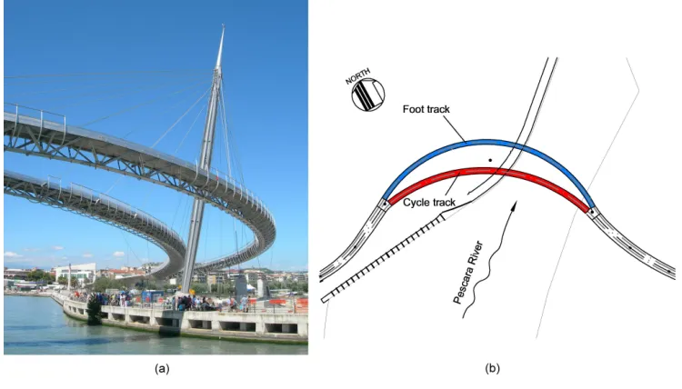
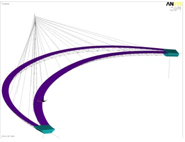
4.2 The ’Ponte del Mare’ bridge in Pescara . . . 62

4.2.1 Description of the Structure . . . 62

4.2.2 FE model . . . 63

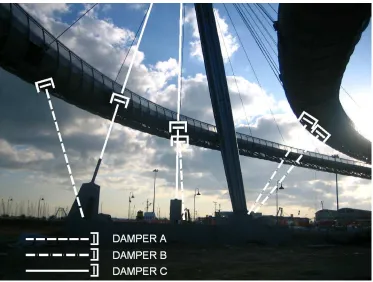
4.2.3 Description of dampers . . . 65

4.3 Design of the dynamic tests . . . 67

4.3.1 Tests set-up . . . 67

4.3.2 Tests in ambient vibration conditions . . . 69

4.3.3 Tests in free-decay conditions . . . 71

4.4 Output-only identification in time domain . . . 71

4.4.1 Modal frequencies . . . 74

4.4.2 Mode shapes . . . 74

4.4.3 Modal damping . . . 78

(9)

4.5 Instantaneous identification of the dampers . . . 82

4.5.1 Structure without dampers . . . 82

4.5.1.1 Ambient vibration tests . . . 82

4.5.1.2 Free decay tests . . . 85

4.5.2 Structure provided with dampers . . . 85

4.5.2.1 Ambient vibration tests . . . 87

4.5.2.2 Free decay tests . . . 90

5 MODEL BASED IDENTIFICATION OF A LARGE CURVED CABLE-STAYED FOOT-CYCLE BRIDGE AND UPDATING TECHNIQUES 97 5.1 Introduction . . . 97

5.2 Model updating techniques . . . 98

5.2.1 Modal reduction and expansion . . . 99

5.2.2 Direct methods and sensitivity (iterative) methods . . . 100

5.2.3 Comparison between identified and analytical data MAC and COMAC . . . 104

5.2.4 Dog-Leg optimisation method . . . 106

5.3 Finite Element model of the foot-cycle bridge ’Ponte del Mare’ Pescara 109 5.3.1 Initial FE model . . . 109

5.3.2 Modified FE model accounting changes during construction . . 116

5.4 Model updating of the foot-cycle bridge ’Ponte del Mare’ Pescara . . . 131

5.4.1 Manual updating . . . 131

5.4.1.1 Selection of parameters . . . 131

5.4.1.2 Calculation of sensitivity matrix . . . 132

5.4.2 Automatic updating: implementation of the method . . . 137

5.5 Results and discussion . . . 142

5.5.1 The final result . . . 142

5.5.2 Applicability of the updated model . . . 172

(10)

6 IDENTIFICATION OF WEAK NONLINEARITIES IN CABLES OF

CABLE-STAYED FOOTBRIDGES 179

6.1 Introduction . . . 179

6.2 Nonlinearity in cable vibration . . . 184

6.2.1 Linearized dynamics of small-sag continuous cable . . . 186

6.2.1.1 Out-of-plane vibration . . . 187

6.2.1.2 In-plane vibration . . . 187

6.2.2 Discrete models of continuous cable for analysis of reduced problems . . . 188

6.2.2.1 Reduced models for 2D dynamics . . . 189

6.3 Higher order dynamic response functions . . . 190

6.3.1 Time domain- IRF . . . 190

6.3.2 Frequency domain- FRF . . . 192

6.4 Non-parametric methods for instantaneous identification of nonlinear systems . . . 193

6.4.1 Identification of Volterra series forms . . . 194

6.4.2 Identification of polynomial forms . . . 196

6.5 Nonlinear identification of cables . . . 199

6.5.1 A numerical example . . . 199

6.6 Results and discussion . . . 202

7 FOOTBRIDGE-PEDESTRIAN INTERACTION 219 7.1 Introduction . . . 219

7.2 A modified hybrid Van der Pol/Rayleigh (MHVR) oscillator for modelling the lateral pedestrian force on a moving floor . . . 220

7.2.1 Pedestrian on a rigid floor . . . 221

7.2.2 Pedestrian on a moving floor . . . 222

7.3 Analytical solution: the harmonic balance method . . . 224

7.3.1 Response curvesν−r2 _{. . . .} ₂₂₇

7.3.2 Analytical vs. numerical results . . . 234

7.4 Stability analysis . . . 235

(11)

7.4.2 Representation in theν−r2_{plane . . . .} ₂₃₉

7.4.3 Representation in theν−λplane . . . 240

7.5 The use of the stability domain for predicting the pedestrian synchro-nization . . . 252

7.5.1 Analytical viewpoint: a 3D normalized synchronization domain 253 7.5.2 Analytical vs. numerical synchronization domain . . . 255

7.5.3 Percentages of synchronization for a group of pedestrians . . . 260

7.6 Phase analysis . . . 262

7.6.1 Phase differenceθbetween relative displacement response and displacement excitation . . . 263

7.6.1.1 Analytical vs. numerical results . . . 263

7.6.2 Phase differenceφ between absolute displacement response and displacement excitation . . . 265

7.6.3 Phase differenceφvfbetween restoring force and external exci-tation (floor) velocity . . . 267

7.7 Effect of frequency and amplitude variations . . . 270

7.8 Numerical vs. experimental results . . . 273

8 SUMMARY, CONCLUSIONS AND FUTURE PERSPECTIVES 279 8.1 Summary . . . 279

(12)

L

IST OF

F

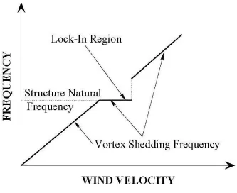
IGURES

2.1 Qualitative trend of vortex shedding frequency with wind velocity during

lock-in (after Simiu and Scanlan 1996) . . . 8

2.2 Wind load (after Kiviluoma 1998) . . . 13

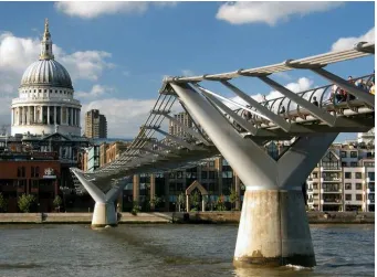
2.3 London Millenium Bridge . . . 19

2.4 Toda Park Bridge, Japan . . . 19

2.5 Periodic walking time histories: vertical and lateral direction (after Zi-vanovic 2005) . . . 23

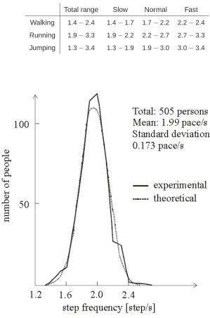
2.6 Normal distribution of pacing frequencies for normal walking (after Mat-sumoto et al. 1978) . . . 24

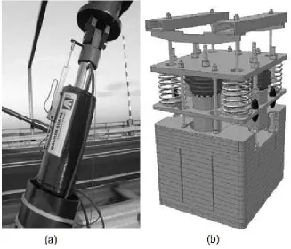
2.7 (a) Absorbing and (b) mass damper . . . 35

4.1 The ’Ponte del Mare’ footbridge . . . 62

4.2 Deck cross-sections. Dimensions in mm . . . 63

4.3 3D FE model of the ’Ponte del Mare’ footbridge . . . 64

4.4 (a) Damper A; (b) Damper C . . . 65

4.5 Dampers location . . . 66

4.6 Accelerometer set-ups used in the dynamic identification tests . . . . 68

4.7 Accelerometer attachments: a) on the deck pavement; b) on a cable . 69 4.8 Ambient vibration time-histories: a) DC1 w/o dampers relative to posi-tion A7 (see Figure 4.6(d)); b)DC1 with dampers relative to posiposi-tion A7 (see Figure 4.6(d)) . . . 70

4.9 Ambient vibration time-histories: a) CP2 w/o dampers relative to posi-tion A10 (see Figure 4.6(e)); b)CP2 with dampers relative to posiposi-tion A10 (see Figure 4.6(e)) . . . 70

(13)

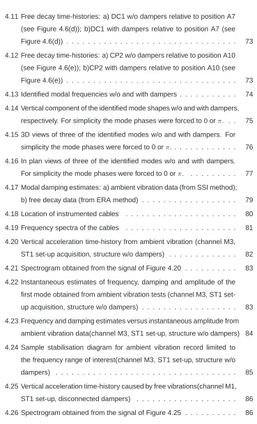
4.11 Free decay time-histories: a) DC1 w/o dampers relative to position A7 (see Figure 4.6(d)); b)DC1 with dampers relative to position A7 (see Figure 4.6(d)) . . . 73 4.12 Free decay time-histories: a) CP2 w/o dampers relative to position A10

(see Figure 4.6(e)); b)CP2 with dampers relative to position A10 (see Figure 4.6(e)) . . . 73 4.13 Identified modal frequencies w/o and with dampers . . . 74 4.14 Vertical component of the identified mode shapes w/o and with dampers,

respectively. For simplicity the mode phases were forced to 0 orπ. . . 75 4.15 3D views of three of the identified modes w/o and with dampers. For

simplicity the mode phases were forced to 0 orπ. . . 76 4.16 In plan views of three of the identified modes w/o and with dampers.

For simplicity the mode phases were forced to 0 orπ. . . 77 4.17 Modal damping estimates: a) ambient vibration data (from SSI method);

b) free decay data (from ERA method) . . . 79 4.18 Location of instrumented cables . . . 80 4.19 Frequency spectra of the cables . . . 81 4.20 Vertical acceleration time-history from ambient vibration (channel M3,

ST1 set-up acquisition, structure w/o dampers) . . . 82 4.21 Spectrogram obtained from the signal of Figure 4.20 . . . 83 4.22 Instantaneous estimates of frequency, damping and amplitude of the

first mode obtained from ambient vibration tests (channel M3, ST1 set-up acquisition, structure w/o dampers) . . . 83 4.23 Frequency and damping estimates versus instantaneous amplitude from

ambient vibration data(channel M3, ST1 set-up, structure w/o dampers) 84 4.24 Sample stabilisation diagram for ambient vibration record limited to

the frequency range of interest(channel M3, ST1 set-up, structure w/o dampers) . . . 85 4.25 Vertical acceleration time-history caused by free vibrations(channel M1,

(14)

4.27 Instantaneous estimates of frequency, damping and amplitude of the first mode obtained from free decay tests (channel M1, ST1 set-up, structure w/o dampers) . . . 87 4.28 Vertical acceleration time-history from ambient excitation(channel M3,

ST1 set-up acquisition, structure with dampers) . . . 88 4.29 Spectrogram obtained from the signal of Figure 4.28 . . . 88 4.30 Instantaneous estimates of frequency, damping and amplitude of the

first mode obtained from ambient vibration tests (channel M3, ST1 set-up acquisition, structure with dampers) . . . 89 4.31 Frequency and damping estimates versus instantaneous amplitude from

ambient vibration data(channel M3, ST1 set-up, structure with dampers) 89 4.32 Sample stabilisation diagram for ambient vibration record limited to

the frequency range of interest(channel M3, ST1 set-up, structure with dampers) . . . 90 4.33 Vertical acceleration time-history caused by free vibrations(channel M1,

ST1 set-up, structure with dampers) . . . 91 4.34 Spectrogram obtained from the signal of Figure 4.33 . . . 92 4.35 Instantaneous estimates of frequency, damping and amplitude of the

first mode obtained from free decay tests (channel M1, ST1 set-up acquisition, structure with dampers) . . . 92 4.36 Mode shape 1 as supplied by the preliminary FE model: a) model with

fully active dampers; b) FE model where the dampers are replaced by their inherent stiffness at small displacements . . . 93 4.37 Comparison of FE vertical component of mode shape 1 with active and

inactive dampers respectively. a) Foot-track deck and b) cycle-track deck. 93 4.38 Frequency and damping estimates versus instantaneous amplitude from

free decay data(channel M1, ST1 set-up, structure with dampers) . . . 94

(15)

5.4 Section types of the elements that constitute the beam reticular(a) Up-per chord (b) Lower chord (c) diagonals, bracings,vertical braces and

dividers. . . 112

5.5 Concrete block as the connection between the pedestrian and cycle deck. . . 115

5.6 Saddle Gerber between concrete block and ramp of access. . . 117

5.7 Progress of the construction work in site. . . 118

5.8 Progress of the construction work in site. . . 119

5.9 Steel-concrete composite secction in zone D of the pedestrian deck. . 119

5.10 Steel-concrete composite secction in zone D’ of the cycle deck. . . 120

5.11 Steel-concrete composite secction of the mast. . . 121

5.12 Detail of the diagonals added in different zones of the pedestrian deck. 122 5.13 Detail of the diagonals added in different zones of the cycle deck. . . . 123

5.14 Arrangement of ALGAFLON support . . . 124

5.15 Arrangements of the cables after final construction . . . 127

5.16 Flow chart to calculate the reduced elastic modulus according to Dischinger theory . . . 129

5.17 Initial MAC in graph . . . 131

5.18 Comparison between the real section D and the shell of FE model . . 132

5.19 Manual sensitivity matrix . . . 134

5.20 Graphical view of the sensitivity matrix . . . 135

5.21 At left a classical view of MAC and at the right difference in MAC values 144 5.22 MAC, xp- experimental & ans- ANSYS . . . 144

5.23 1st mode of ANSYS correlated with 1st mode of experiment with MAC=98.6 146 5.24 Normalized vertical autovector of the pedestrian deck . . . 147

5.25 Normalized vertical autovector of the cycle deck . . . 147

5.26 Normalized radial autovector of the pedestrian deck . . . 148

5.27 2nd mode of ANSYS correlated with 2nd mode of experiment with MAC=42.5 . . . 149

5.28 Normalized vertical autovector of the pedestrian deck . . . 150

(16)

5.31 Normalized radial autovector of the cycle deck . . . 151

5.32 3rd mode of ANSYS correlated with 3rd mode of experiment with MAC=76.8152 5.33 Normalized vertical autovector of the pedestrian deck . . . 153

5.37 4th mode of ANSYS correlated with 4th mode of experiment with MAC=94.8155 5.38 Normalized vertical autovector of the pedestrian deck . . . 156

5.57 12th mode of ANSYS correlated with 10th mode of experiment with MAC=60.4 . . . 167

(17)

5.61 13th mode of ANSYS correlated with 11th mode of experiment with

MAC=48.7 . . . 170

5.65 Position of the two anemometers, (a) below the pedestrian deck, (b) at the top of the mast . . . 173

5.66 The wind speed from the two annemometers . . . 174

5.67 comparison between the acceleration recorded at M1 with the vertical acceleration at node 11003 of ANSYS model without dampers . . . . 175

5.68 comparison between the acceleration recorded at M3 with the vertical acceleration at node 11042 of ANSYS model without dampers . . . . 175

5.69 comparison between the acceleration recorded at M1 with the vertical acceleration at node 11003 of ANSYS model with dampers . . . 176

5.70 comparison between the acceleration recorded at M3 with the vertical acceleration at node 11042 of ANSYS model with dampers . . . 176

6.1 Typical response of cable-stay bridges after (Abdel-Ghaffar and Nazmy, 1991) . . . 180

6.2 Classification of the nonlinear identification methods . . . 183

6.3 Cable configurations and displacement components in a global refer-ence system, after (Rega, 2004a) . . . 184

6.4 Input-output diagram . . . 191

6.5 Cable element of example . . . 199

6.6 Force-displacement relation . . . 203

6.7 Time variation of the parameters for P0= 0.5kN. . . 203

6.8 Displacement response for P0= 0.5kN . . . 204

6.9 FFT of the displacement response, P0= 0.5kN . . . 204

6.10 Time variation of the parameters for P0= 5kN . . . 205

6.11 Displacement response for P0= 5kN . . . 205

6.12 FFT of the displacement response, P0= 5kN . . . 206

(18)

6.29 Variation of mean values of parameters vs. P0. . . 215

7.1 (a) Scheme of the Two-DoF system representing the coupled lateral motion of a pedestrian and the deck of a footbridge. (b) Single-DoF oscillator representing a pedestrian on a floor undergoing a harmonic motion. . . 223

7.2 Response curves of the MHVR oscillator: (a) isochronous case (α= 0) and (b) non-isochronous case (example withα= 2). The curves show the real and positive solutions of Eq. (7.15). Dashed line: λ=0.15 , dotted line:λ=0.35 , solid line:λ=1.0 . . . 228

7.3 Response curves and stability regions of the MHVR oscillator. Dotted lines: response amplitude curves associated with Eq. (7.20). Contin-uous lines: conic associated with the saddle-node bifurcation (7.44). Dashed-dotted lines: Hopf bifurcation (7.45). Dashed lines: nodes-spirals bifurcation (7.46). . . 230

(19)

7.5 Response curves of the MHVR oscillator (Eq. (7.15)) forα = 1and with five differentλ-values. The vertical line corresponds toν = 1.4492, while the dashed ellipse is associated with the condition (7.23). . . 232

7.6 Response curves of the MHVR oscillator (Eq.(7.15)) forα= 1. Com-parison between numerical and analytical results for three differentλ -values. . . 236

7.7 Bifurcations portraits of the MHVR oscillator in the parameter plane (ν,λ). Caseα= 0.Global view and detail of the zone around the right cusp A of the saddle-node bifurcation BS. . . 242

7.8 Bifurcations portraits of the MHVR oscillator in the parameter plane (ν,λ). Caseα= 0.5. . . 243

7.9 Bifurcations portraits of the MHVR oscillator in the parameter plane (ν,λ). Caseα = 1.Global view and (a) detail of the zone around the left cusp of BS; (b) detail of the zone inside BSwhere the branches of

the node-spiral bifurcation BN intersect; (c) detail of the zone around

the right cusp of BS. . . 244

7.10 Bifurcations portraits of the MHVR oscillator in the parameter plane (ν,λ). Caseα= 2.. . . 245

7.11 Surface representing the lower boundary of the stability domain, ac-cording to the analytical approximation defined in Table 7.5. Each point

over the surface represents a pedestrian synchronized with the

har-monically moving floor. . . 251

7.12 Comparison between the analytical and numerical estimations of the boundary of the stability domain of the MHVR oscillator. Caseα= 0. . 256

7.13 Comparison between the analytical and numerical estimations of the boundary of the stability domain of the MHVR oscillator. Caseα= 0.5. 257

(20)

7.15 Time-evolution of the displacements of the center of mass of pedes-trian ”2” (vx = 3.75 km/h Erlicher et al. (2010)) in the case of (a) non-entrained oscillation (Aacc = 0.05 m/s2, ω/(2π) = 1 Hz) and (b) entrained oscillation (Aacc = 0.15 m/s2, ω/(2π) = 1Hz). uy :relative

displacement; Uy+uy : absolute displacement; Uy : shake table

dis-placement. . . 259 7.16 Analytical and numerical comparison of the phase difference between

relative displacement response and and displacement excitation for

α= 1.andλ= 0.35, 1.5and 2.5 . . . 264 7.17 Analytical and numerical comparison of the phase difference between

absolute displacement response and displacement excitation forα= 1 andλ= 0.35, 1.5and 2.5 . . . 266 7.18 Analytical and numerical comparison of phase difference between

lat-eral force and floor velocity. Forα= 1.andλ= 0.35, 1.5and 2.5 . . . . 269 7.19 Pedestrian ”2”- effect of varying frequency (f ) and amplitude (Ad) on (a)

φ(b)φvf . . . 271

7.19 Pedestrian ”2”- effect of varying frequency (f ) and amplitude (Ad) on (c)

R/Ad(d) A/Ad . . . 272

7.20 Displacement and force-time plot for pedestrian no. ”2” at floor excita-tion amplitude 3 cm and frequency 1 Hz . . . 274 7.21 Displacement and force-time plot for pedestrian no. ”5” at floor

(21)

L

IST OF

T

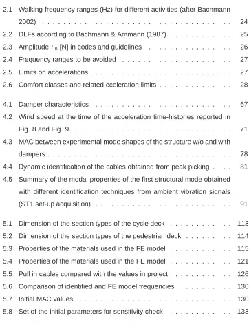
ABLES

2.1 Walking frequency ranges (Hz) for different activities (after Bachmann

2002) . . . 24

2.2 DLFs according to Bachmann & Ammann (1987) . . . 25

2.3 Amplitude F0[N] in codes and guidelines . . . 26

2.4 Frequency ranges to be avoided . . . 27

2.5 Limits on accelerations . . . 27

2.6 Comfort classes and related cceleration limits . . . 28

4.1 Damper characteristics . . . 67

4.2 Wind speed at the time of the acceleration time-histories reported in Fig. 8 and Fig. 9. . . 71

4.3 MAC between experimental mode shapes of the structure w/o and with dampers . . . 78

4.4 Dynamic identification of the cables obtained from peak picking . . . . 81

4.5 Summary of the modal properties of the first structural mode obtained with different identification techniques from ambient vibration signals (ST1 set-up acquisition) . . . 91

5.1 Dimension of the section types of the cycle deck . . . 113

5.2 Dimension of the section types of the pedestrian deck . . . 114

5.3 Properties of the materials used in the FE model . . . 115

5.4 Properties of the materials used in the FE model . . . 121

5.5 Pull in cables compared with the values in project . . . 126

5.6 Comparison of identified and FE model frequencies . . . 130

5.7 Initial MAC values . . . 130

(22)

5.9 Set of parameters used in model updating . . . 136 5.10 Range of the admissibility of the parameters . . . 141 5.11 Set of parameters that minimize the difference with the experimental

frequency . . . 142 5.12 Frequencies obtained at the end of model updating and mean

percent-age error comes 2.89% . . . 143 5.13 Updated MAC values . . . 143 5.14 Difference in acceleration RMS values recorded and from FE model

with and without dampers . . . 177

6.1 Properties of the cable . . . 200 6.2 Modal frequencies . . . 200 6.3 Identified parameters: mean value, standard deviation (sd) and

coeffi-cient of variation (cv %) . . . 214 6.4 Frequencies obtained from the FFT of the response . . . 215

7.1 Coordinates (z,ν,λ)of the points O and O0_{, at the intersection of B}_S_,

BHand BN. . . 241

7.2 Coordinates z and (ν,λ)of the cusp points of the saddle-node bifurca-tion BS. . . 243

7.3 Description of the fixed points in the different regions of the bifurcation diagrams. First part. (s.n.=stable node; s.s.= stable spiral; sd.= saddle; u.n.= unstable node; u.s.= unstable spiral). . . 248 7.4 Description of the fixed points in the different regions of the bifurcation

diagrams. Second part. (s.n.=stable node; s.s.= stable spiral; sd.= saddle; u.n.= unstable node; u.s.= unstable spiral). . . 249 7.5 Inequalities defining the stability domain for the entrained solutions

(7.6)-(7.10) of the non-autonomous MHVR oscillator (7.5), according to the analytical approximation based on the harmonic balance method.

λQ=λQ(α,ν)andλH=λH(α,ν)are defined by Eqs. (7.48) and (7.49),

(23)

7.6 Percentages of synchronized pedestrians in a population of twelve people. The average of the natural walking frequencies of all pedestri-ans is ¯f1= 0.848Hzwith a standard deviation of 0.055 Hz. . . 261

7.7 Percentages of synchronized pedestrians in a population of twelve people. The average of the natural walking frequencies of all pedestri-ans is ¯f1= 0.923Hzwith a standard deviation of 0.053 Hz. . . 261

(24)

(25)

C

HAPTER

1

INTRODUCTION

Bridges are indispensable components of the infrastructure of modern society. They are of many different types, e.g. beam, arch, cantilever, suspension, cable-stayed etc., depending on application and design. Compared to other bridge types, the cable-stayed bridges (CSB) are optimal for spans longer than typically seen in can-tilever bridges and shorter than those typically requiring a suspension bridge. Cable-stayed bridges mainly consist of cables, pylons and girders (bridge decks).

Due to their aesthetic appearance, efficient utilization of structural materials and other notable advantages, cable-stayed bridges have gained much popularity in re-cent decades. Nowadays, as their properties have been more fully understood, very long span slender cable-stayed bridges are being built, and the ambition is to fur-ther increase the span length and use shallower and more slender girders for future bridges. Bridges of this type are entering a new era with main span lengths reaching 1000 m, e.g. Sutong CSB in China spans 1088 m (Janjic). This fact is due to the relatively small size of the substructures required, the development of efficient con-struction techniques and the rapid progress in the analysis and design of this type of bridges. They have recently proved to be highly cost-effective for short to medium spans.

(26)

1995)- with a single inclined pylon; the Safti Link Bridge (Brownjohn and Xia, 2000)-which has a curved deck and single offset pylon; circular cable stayed footbridge (Rebelo et al., 2010) and twin curved deck footbridges (Gentile et al., 2004; Tondini et al., 2010). The unique structural styles of these bridges beautify the environment, however, add to the difficulties in accurate structural analysis due to their complex shape. It is, therefore necessary to perform experimental identification tests to mea-sure the actual dynamic properties, for e.g. resonant frequency, mode shape and modal damping, of the bridges to understand better their dynamic behavior. These measured properties can be used to correct and update numerical FE model to better reflect the reality. The updated FE model can be useful to predict the damage and safety conditions of the bridge under the extreme loading events, such as typhoon or earthquake.

For cable supported bridges and in particular long span cable-stayed bridges, en-ergy dissipation is very low and is often not enough on its own to suppress vibrations (Forsterling and Furtner, 2004; Hikami, 1986). To increase the overall damping ca-pacity of the bridge structure, one possible option is to incorporate external dampers, i.e. discrete damping devices such as viscous dampers and MR dampers, into the system. Such devices are frequently used nowadays for cable supported bridges. However, it is not believed that this is always the most effective and the most eco-nomic solution. Therefore, a great deal of research is needed to investigate the damping capacity of modern cable-stayed bridges and to find new alternatives to in-crease the overall damping of the bridge structure. Moreover, it is deemed necessary to investigate the effectiveness of the dampers after installing on the bridge.

Modern cable-stayed bridges exhibit geometrically nonlinear behaviour, they are very flexible and undergo large displacements before attaining their equilibrium con-figuration. Stay cables impart major part of the geometrical nonlinearity in the global dynamics; a well known deck-cable interaction phenomenon was reported by several researchers in cable-stayed footbridges (Caetano et al., 2000, 2008). To identify the nonlinear behaviour of the cables from the response data, special techniques are required.

(27)

slen-der footbridges. Therefore, the moslen-dern cable-stayed footbridges have become more prone to vibrations due to the wind and pedestrian actions. The very large ampli-tude lateral vibrations of Millenium bridge (Dallard et al., 2001a) decks on its open-ing day 10 June 2000, has realized the complexity of the serviceability problems in pedestrian-footbridge interaction. Several researchers have introduced models to ex-plain the phenomenon of synchronous lateral excitation of footbridges, but there is no consensus on the general applicability of these models. Hence, there is still ef-fort to model the pedestrian-footbridge behaviour in order to understand this complex phenomenon.

1.1 Objectives of the research

As discussed in the previous section, modern cable-stayed bridges are made in distinctive styles, that adds complexity to the structure. However, flexible, slender and lighter CSB are more prone to wind- and pedestrian- induced vibrations. A performance-based approach of cable-stayed footbridges requires the consideration of both ultimate as well as serviceability limit states. Even though a footbridge may be endowed with a robust design against failure, serviceability problems may arise from many sources, such as wind, pedestrians, nonlinear behaviour of cables and their interaction to the deck, ineffectiveness of damper system, etc. A more complete approach towards the investigation of the performance of a cable-stayed footbridge was considered in this thesis.

(28)

1.2 Structure of the thesis

This thesis presents the research work performed by the author on the system iden-tification and pedestrian-induced vibration of cable-stayed footbridges. The research was sponsored by “HITUBES: Design and Integrity Assessment of High Strength Tubular Structures for Extreme Loading Conditions”- a Research Fund for Coal and Steel (RFCS) funded project of the European Commission to the University of Trento. The second chapter provides the state of the art on the dynamic response of cable-stayed footbridges (CSFB). As the CSFB are mainly subjected to wind and pedestrian loadings in their everyday life, the review focuses on the dynamic response of the CSFB due to wind and anthropic actions. Moreover, it also discusses some damping system applicable to the main deck as well as stay cables.

Structural identification techniques are summarised in chapter 3. Both linear and nonlinear techniques are reviewed. Then, techniques relevant to cable-stayed foot-bridges are described.

In chapter 4, the design and outcomes of the dynamic identification tests of the ‘Ponte del mare’ footbridge are described. Moreover, the instantaneous identification is performed in order to investigate the effectiveness of the installed dampers.

The model updating is carried out on the FE model in view of the measured identifi-cation data in chapter 5. The updated model is used to simulate the actual behaviour of the footbridge under a measured wind excitation.

In chapter 6, the numerical analysis is carried out to investigate the applicability of time-frequency techniques for the nonlinear identification of cables.

The pedestrian-footbridge behaviour is analytically modelled and numerical com-parisons are made in chapter 7.

(29)

C

HAPTER

2

DYNAMIC RESPONSE OF CABLE-STAYED FOOTBRIDGES: A

STATE-OF-THE-ART

2.1 Introduction

Footbridges are mainly subjected to the action of the wind and pedestrians in their everyday life. This chapter reviews the literature concerning the three aspects of the cable-stayed footbridges (CSB): i) dynamic response due to the wind; ii) dynamic response due to pedestrians; and iii) vibration reduction techniques for cable-stayed footbridges. Factors affecting the behaviour of bridges are discussed, both due to the wind and pedestrians. Finally, some vibration reduction techniques are reviewed.

(30)

2.2 Dynamic response due to the wind

2.2.1 Wind loading phenomena

The criteria for the design of long spanned cable-stayed bridges are concerned with the static and dynamic responses of the bridge under wind loading. The design of long span bridges is often governed by aeroelastic instability. Aerodynamic design involves calculation of the critical velocity for the onset of flutter. It is to be ensured that the wind velocity does not exceed the predicted critical velocity to avoid failure due to flutter (Selvam and Govindaswamy, 2001). A list of bridges failure due to the wind can be found in (Rutz and Rens, 2007).

Arrol and Chatterjee (Arrol and Chatterjee, 1981) mention that designers should remember that the position of maximum stress would not always be at mid-span, or a support, and the stress value will depend upon the mode shape. In a simply supported span the second mode maximum stress is at the quarter points and will have a value four times that of the fundamental mode maximum stress, occurring at mid span.

When designing a bridge, one has to take into account the wind effects on the structure. Wind loading can be categorised into two categories; Static and dynamic wind loading. Static wind load is the most basic wind effect considered when de-signing a structure. For bridges, the static behaviour is less critical to the dynamic effects. There are many types of dynamic wind load. The one that will be addressed are buffeting, vortex shedding, galloping, torsional divergence, and flutter.

Dynamic behavior includes the responses due to vortex shedding excitation, self-excited oscillations and buffeting by wind turbulence (Selvam, 1998). Bridges could oscillate in two natural modes, vertical and torsional. In the vertical mode, all joints at any cross-section move the same distance in the vertical plane, while in the torsional mode every cross-section rotates about a longitudinal axis parallel to the roadway.

(31)

understand the issues involved in the design is explained in the following sub-section.

2.2.1.1 Aeroelastic Instability

Aeroelasticity is the discipline concerned with the study of phenomena wherein the aerodynamic forces and structural motions interact significantly. When a structure is subjected to wind flow, it may vibrate or suddenly deflect in the airflow. This structural motion results in a change in the flow pattern around the structure. If the modification of wind pattern around the structure by aerodynamic forces is such that it increases rather than decreasing the vibration, thereby giving rise to succeeding deflections of oscillatory and/or divergent character, aeroelastic instability is said to occur (Simiu and Scanlan, 1996). The aeroelastic phenomena that are considered in wind engi-neering are vortex shedding, torsional divergence, galloping, flutter and buffeting.

Vortex Shedding

Simiu and Scanlan (Simiu and Scanlan, 1996) state that when a body is subjected to wind flow, the separation of flow occurs around the body. This produces force on the body, a pressure force on the windward side and a suction force on the leeward side. The pressure and suction forces result in the formation of vortices in the wake region causing structural deflections on the body. The shedding of vorticity balances the change of fluid momentum along the entire body surface. The shed vortices are convected downwind by local mean wind speed and viscous diffusion but will also interact to form large-scale coherent structures. The frequency in which the vortices are shed dictates the structural response. The structural member acts as if rigidly fixed, when the frequency of vortex shedding (also called wake frequency) is not close to the natural frequency of the member. On the other hand, when the vortex-induced and the natural-frequencies coincide, the resulting condition is called lock-in. During lock-in condition, the structural member oscillates with increased amplitude but rarely exceeding half of the across wind dimension of the body (Simiu and Scanlan, 1996). The lock-in condition is illustrated in Figure 2.1.

(32)

(33)

defined as:

Re = ρUD

µ (2.1)

St=

NsD

U (2.2)

where,ρ= wind density, U = wind velocity, D = diameter,µ= viscosity, and Ns = frequency of vortex cycle shedding.

For a very low Reynolds number (Selvam and Govindaswamy, 2001; Simiu and Scanlan, 1996) the flow remains the same, just circumventing the obstruction on its way. For higher Reynolds numbers, the flow starts to separate around the edges of the obstruction and vortices are generated in the immediate wake of the obstruc-tion. Thereafter further increase in the Reynolds number causes the creation of cycli-cally alternating vortices and they are carried over with the flow downstream. From there on, the inertial effects become dominant over the viscous effects and turbulence sets in, resulting in shear of the flow. So this reasonably illustrates the vorticity phe-nomenon starting from a smooth and low speed flow to a turbulent and high-speed flow.

Galloping

Simiu and Scanlan (Simiu and Scanlan, 1996) state that galloping is an instabil-ity typical of slender structures. This is a relatively low-frequency oscillatory phe-nomenon of elongated, bluff bodies acted upon by a wind stream. The natural struc-tural frequency at which the bluff object responds is much lower than the frequency of vortex shedding. It is in this sense that galloping may be considered a low-frequency phenomenon. There are two types of galloping: Wake and Across-wind.

(34)

Across wind galloping: Across wind galloping in a bridge, is an instability that is initi-ated by a turbulent wind blowing transversely across the deck. Across-wind galloping causes a crosswise vibration in the bridge deck (Liu, 1991). As the section vibrates crosswise in a steady wind velocity (U), the relative velocity changes, thereby chang-ing the angle of attack (α). Due to the change in α, an increase or decrease on the lift force of the cylinder occurs. If an increase ofαcauses an increase in the lift force in the opposite direction of motion, the situation is stable. But on the other hand if the vice versa occurs, i. e., an increase ofαcauses a decrease in lift force, then the situation is unstable and galloping occurs.

Torsional divergence

Torsional divergence is an instance of a static response of a structure. Torsional divergence was at first associated with aircraft wings due to their susceptibility to twisting off at excessive air speeds (Simiu and Scanlan, 1996). Liu (Liu, 1991), re-ports that when the wind flow occurs, drag, lift, and moment are produced on the structure. This moment induces a twist on the structure and causes the angle of inci-denceαto increase. The increase inαresults in higher torsional moment as the wind velocity increases. If the structure does not have sufficient torsional stiffness to resist this increasing moment, the structure becomes unstable and will be twisted to failure. Simiu and Scanlan (Simiu and Scanlan, 1996) report that the phenomenon depends upon structural flexibility and the manner in which the aerodynamic moments develop with twist; it does not depend upon ultimate strength. They say that in most cases the critical divergence velocities are extremely high, well beyond the range of velocities normally considered in design.

Flutter

The phenomenon of flutter (classical flutter) is a very serious concern in the design of bridges. The failure of the Tacoma’s narrows bridge was due to the flutter. The term flutter has been variously used to describe different types of wind-induced behavior. Flutter can be defined as a condition of negative aerodynamic damping wherein the deflection in the structure grows to enormous levels till failure once started. The other types of flutter reported by Simiu and Scanlan (Simiu and Scanlan, 1996) are stall flutter and panel flutter.

(35)

nonlinear characteristics of the lift (Simiu and Scanlan, 1996). The stall flutter phe-nomenon can also occur with structures having broad surfaces depending on the angle of approaching wind. The torsional oscillation of a traffic stop sign about its post is an example of this phenomenon.

Panel flutter is a sustained oscillation of panels typically the sides of large rock-ets, caused by the high-speed passage of air along the panel. The most prominent cases have been in supersonic flow regimes and so have not appeared in the wind engineering context. Flag flutter is closely related to panel flutter.

The motion that is caused by the wind flow will either be damped out or will grow indefinitely until failure. The theoretical dividing line between these two states is the critical flutter condition and the wind speed at this condition is called critical wind speed.

Critical wind speeds for Flutter

When the critical wind speed for flutter is exceeded, the structure will become un-stable and experience excessive deflections. Hence it is an important factor to be considered in design. Arrol and Chatterjee (Arrol and Chatterjee, 1981) mention the following guidelines.

Vortex shedding: With respect to vortex shedding, if the critical wind speed for reso-nance in vertical and torsional modes (vertical modes only for trusses) is greater than the reference wind speed, the static and fatigue stress effects need to be checked from amplitude calculations appropriate to the mode shape.

Turbulence Response: If the natural frequency in first mode for vertical or torsional deflection is greater than 1 Hz, a dynamic analysis for stress effects need to be carried out to account for it.

Classical and Stall flutter: For prevention of this type of instability, the critical wind speed is to be greater than 1.3 times reference speed. The designer must ensure one of the following. The critical wind speed exceeds the practical limiting value for the given site or the resulting amplitudes are of allowable levels. Criteria for accept-ability may include considerations of fatigue or of user reaction as well as of ultimate strength.

Buffeting

(36)

in the incoming flow and not self-induced (Simiu and Scanlan, 1996). Buffeting vi-bration is the vivi-bration produced by turbulence. There are two types of buffeting. One type is caused by turbulence in the airflow, and the other type is caused by dis-turbances generated by an upwind neighboring structure or obstacle. The first type of buffeting can produce significant vertical and torsional motions of a bridge even at low speeds. This buffeting induced motion results in a gradual transition to large amplitude torsional oscillations, which could lead to the failure of a bridge. If the ve-locity fluctuations are clearly associated with the turbulence shed in the wake of an upstream body, the unsteady loading is referred to as wake buffeting. Wake buffeting is common in urban areas with many tall structures.

2.2.1.2 Wind load model

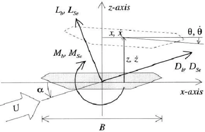
The aerodynamic loads acting on a body can be divided into static (St), buffeting (b) and self-excited (Se) parts by the formula (Kiviluoma, 1998)

        

L = Lst+Lb+Lse

D = Dst+Db+Dse

M = Mst+Mb+Mse

(2.3)

in which L , D and M are the time dependent lift, drag and (pitching) moment, re-spectively.

Applying the dimensionless steady aerodynamic lift CL, drag CD, and moment CM

coefficients of a typical cross-section (Fig. 2.2) the static terms are (Kiviluoma, 1998)

        

Lst = 1₂ρU2BlCL

Dst= 1₂ρU2BlCD

Mst = 1₂ρU2BlCM

(2.4)

(37)

Figure 2.2: Wind load (after Kiviluoma 1998)

by the corresponding transverse fluctuating velocity component w(t). In Eq. 2.3 the buffeting terms take into account the fluctuations in wind speed and direction relative to a body at rest while the self-excited forces take into account the aerodynamic forces caused by motion of the body itself. The approximationsα≈w/Uand Ci(α)_≈Ci +α

dCi/dα,(i = C, D or M) yield the widely used quasi-steady formulation for the buffeting terms (Kiviluoma, 1998)

        

Lb=ρUBl(CLu +1₂dC_d_αLw)

Db=ρUBl(CDu +1₂dC_d_αDw)

Mb=ρUB2l(CMu +1₂dC_d_αMw)

(2.5)

whereαis the angle of attack. Using the typical American notation of flutter deriva-tives and applying the sign convention of Fig. 2.2, the self-excited terms for sinusoidal motion can be expressed by the formula (Kiviluoma, 1998)

        

Lse= 1₂ρU2Bl(KH∗1 z

U +KH2∗

Bθ

U +K

2_H_∗

3θ+K

2_H_∗ 4 z

B)

Dse= 1₂ρU2Bl(KP1∗Ux +KP2∗BUθ +K 2_P_∗

3θ+K2P4∗Bx)

Mse= 1₂ρU2B2l(KA1∗ z

U +KA2∗

Bθ

U +K

2_A_∗

3θ+K2A4∗ z

B)

(38)

in which the flutter derivatives and Pi, Hiand Ai (i=1, 2, 3 or 4) are functions of the

reduced frequency K = Bω/U only, whereω is the circular frequency of the motion. The notation used here is the same as that used in (Scanlan, 1993) except the pos-itive direction of the vertical coordinate z and the vertical force component L . Thus, flutter derivatives H2, H3, A1and A4possess negative signs compared to American

literature.

In Eq. 2.6 no terms proportional to translational or rotational accelerations are given and thus the effect of the apparent mass of fluid is neglected. This restricts the usage of the equation to structural members that are relatively dense in comparison to the density of the fluid. Furthermore, usage of the mean wind velocity in Eq. 2.6 implies some inconsistency in analysis of wind-speeds just below the flutter velocity, since the latter velocity is probably exceeded in short duration gusts.

2.2.2 Wind effect on bridges

Wind loading has long played a significant role in bridge design. Some spectacu-lar failures, such as the Tay Bridge (Scotland, 1879), or the Tacoma Narrow Bridge (Washington state,1940) acted as painful reminder to the engineers in case they had forgotten the importance of wind loading. Very long span cable-stayed bridges are flexible structural systems. These flexible systems are susceptible to the dynamic effects of wind loads. Wind can produce the following effects on cable-stayed bridges (Farran, 1999):

1. Wind lift and drag forces,

2. Aeroelastic effects (torsional divergence or lateral buckling), 3. Oscillations induced by vortex effects,

4. Flutter phenomena, 5. Galloping effects, and 6. Buffeting.

(39)

bridge. There are 3 types of wind tunnel tests on a suspension bridge:

1. Models of the entire bridge,

2. Taut strip models, and

3. Sectional models.

The first category of wind tunnel models provides the engineer with the advan-tages of similitude between model and prototype. These models are expensive to build and constitute a large initial capital expenditure. Experience from previous de-signs indicates that a scale of 1 to 300 is desirable. Other scales are also possible. The distribution of the mass in such complete scale models is identical to the mass distribution of the real life structure or prototype.

The second category, or the taut strip model, consists of 2 wires that are stretched across the wind tunnel. The response of such models to applied fluid flows in the wind tunnel is similar to the response of the center section of the suspension structure.

The third category is made up of sections of the bridge deck in the span-wise direction. The ends of these sections are supported on spring type foundations to allow motion in the vertical direction as well as the rotational sense. The usual scales for such deck sections are within the 1/50 to 1/25 range. These sectional models are very important in determining the aeroelastic stability of the proposed deck system. These models allow us to further investigate the steady state coefficients for drag, lift, and moment.

(40)

2.2.3 Wind effect on stay cables

Stay cables are susceptible to wind (and rain) induced vibration in cable-stayed bridges. Matsumoto et al. (Matsumoto et al., 1992) observed double amplitude (peak to peak) on the Bridge Islands (Denmark) up to 2 m due to the combined effect of rain and wind.

There are a number of mechanisms that can potentially lead to vibrations of stay cables. Some of these types of excitation are more critical or probable than others but all are listed here for completeness (Kumarasena et al., 2005):

•Vortex excitation of an isolated cable;

•Vortex excitation of groups of cables;

•Wake galloping for groups of cables;

•Galloping of single cables inclined to the wind;

•Rain/wind-induced vibrations of cables;

•Galloping of cables with ice accumulations;

• Galloping of cables in the wakes of other structural components (e.g., arches, towers, truss members);

•Aerodynamic excitation of overall bridge modes of vibration involving cable motion (e.g., vortex shedding off the deck may excite a vertical mode that involves relatively small deck motions but substantial cable motions);

•Motions caused by wind turbulence buffeting; and

•Motion caused by fluctuating cable tensions.

For a detail discussion of the above mechanisms of stay cables, the reader can refer to the FHWA report (Kumarasena et al., 2005). The FHWA report, a first report, that provides a design guidelines for the mitigation of wind-induced vibrations of stay cables. FHWA report concludes its initial review with that- while the rain/wind problem is known in sufficient detail (Phelan et al., 2006), galloping of dry inclined cables was the most critical wind-induced vibration mechanism in need of further experimental research.

Rain-wind vibrations

(41)

cable-stayed bridges and has been researched in detail. Rain/wind-induced vibra-tions were first identified by Hikami and Shiraishi on the Meiko-Nishi cable-stayed bridge (Hikami, 1986). Since then, these vibrations have been observed on other cable-stayed bridges, including the Fred Hartman Bridge in Texas, the Sidney Lanier Bridge in Georgia, the Cochrane Bridge in Alabama, the Talmadge Memorial Bridge in Georgia, the Faroe Bridge in Denmark, the Aratsu Bridge in Japan, the Tempohzan Bridge in Japan, the Erasmus Bridge in Holland, and the Nanpu and Yangpu Bridges in China. These vibrations occurred typically when there was rain and moderate wind speeds (8–15 m/s) in the direction angled 20◦ _{to 60}◦ _{to the cable plane, with the}

cable declined in the direction of the wind. The frequencies were low, typically less than 3 Hz. The peak amplitudes were very high, in the range of 0.25 to 1.0 m, violent movements resulting in the clashing of adjacent cables observed in several cases (Kumarasena et al., 2005).

Wind tunnel tests have shown that rivulets of water running down the upper and lower surfaces of the cable in rainy weather were the essential component of this aeroelastic instability(Hikami, 1986). The water rivulets changed the effective shape of the cable and moved as the cable oscillated, causing cyclical changes in the aero-dynamic forces which led to the wind feeding energy into oscillations. The following criterion can be used to specify the amount of damping that must be added to the cable to mitigate rain/wind-induced vibrations:

Sc=

mζ

ρd2 >10 (2.7)

where, Sc= Scruton number, m = mass of cable per unit length (kg/m),ζ= damping

as ratio of critical damping,ρ= air density (kg/m3_{), and d = cable diameter (m).}

(42)

corresponds to a Scruton number of approximately 3, which is less than the minimum of 10 established for suppression of rain/wind vibrations (Eq. 2.7). Therefore dry cable instability should be suppressed by default if enough damping is provided to mitigate rain/wind vibrations.

2.3 Dynamic response due to pedestrians

Although there have been several cases of footbridges experiencing excessive vi-brations by pedestrians in the past, this problem attracted considerably greater public and professional attention only after the infamous swaying of the London Millennium Footbridge located across the Thames River in Central London, see Figure 2.3. The Millennium Bridge problem attracted more than 1000 press articles and over 150 broadcasts in the media around the world (Zivanovic et al., 2005).

The bridge was opened to the public on 10 June 2000 and during the first day be-tween 80,000 and 100,000 people crossed the bridge, resulting in a maximum crowd density of between 1.3 - 1.5 persons per square meter at any one time (Dallard et al., 2001a). On the first day, the Millennium Bridge experienced horizontal vibrations in-duced by a synchronized horizontal pedestrian load. The horizontal vibrations took place mainly on the south span, at a frequency of around 0.8 Hz and on the cen-tral span, at frequencies of just under 0.5 Hz and 0.9 Hz, the first and second lateral modes respectively (Dallard et al., 2001a). The oscillations had maximum amplitudes of 50mm on the southern span and 70 mm on the central span (Dallard et al., 2001b). The maximum lateral acceleration of the bridge was estimated to be between 1.9 and 2.45 ms−2_{.The bridge’s lateral movements caused many pedestrians to have difficulty}

(43)

Figure 2.3: London Millenium Bridge

(44)

One of the earliest reported incidences of excessive horizontal vibrations due to synchronized horizontal pedestrian load occurred on the Toda Park Bridge (T-bridge), Toda City, Japan (Fujino et al., 1993; Nakamura and Fujino, 2002). The T-bridge is a pedestrian cable-stayed bridge which was completed in 1989. It has a main span of 134 meters, a side span of 45 meters, and two cable planes with 11 stays per plane, see Figure 2.4. It was observed that several stays and the girder vibrated when a large number of people (some 2000) were crossing the T-bridge after big boat races. The girder vibrated laterally with amplitude of about 10 mm and a frequency of about 0.9 Hz, the natural frequency of the first lateral mode. Although this amplitude does not seem to be large, some pedestrians felt uncomfortable and unsafe (Fujino et al., 1993; Nakamura and Fujino, 2002; Nakamura, 2004). By video recording and observing the movement of people’s heads in the crowd, and by measuring the lateral response, Fujino et al. (Fujino et al., 1993) concluded that 20% of the people in the crowd perfectly synchronized their walking.

In 1975, the north section of the Auckland Harbour Road Bridge in New Zealand, experienced lateral vibrations during a public demonstration, when the bridge was being crossed by between 2000 and 4000 demonstrators. The span of the north section is 190 meters and the bridge deck is made of a steel box girder. Its lowest natural horizontal frequency is 0.67 Hz (Dallard et al., 2001a).

In addition, horizontal vibrations were among several reasons behind the closure of the Solferino Bridge in Paris immediately after its opening in December 1999. Also, a 100 year-old footbridge, Alexandra Bridge in Ottawa, experienced strong lateral vi-brations in July 2000, when subjected to crowd loading by spectators of a fireworks display (Dallard et al., 2001b). Other types of bridges such as conventional sus-pension bridges such as the Groves Sussus-pension Bridge in Chester have also been reported to experience similar lateral vibrations (Dallard et al., 2001a).

(45)

lateral vibration. The reason for this is that the range of footbridge natural (lateral) fre-quencies often coincides with the dominant frefre-quencies of the human-induced load (Zivanovic et al., 2005). It is therefore stated, that pedestrians can induce excessive lateral vibrations on a footbridge of any structural form, if there is a lateral natural frequency below or near to the lateral human loading frequency – for e.g. about 1 Hz, in case of walking.

2.3.1 Synchronous Lateral Excitation (SLE)

When a pedestrian walks on a lively footbridge human-structure interaction can occur. The interaction takes place in two ways (Venuti and Bruno, 2010). First of all, the presence of the pedestrians modifies the bridge dynamic properties. A first effect is the change of natural frequencies due to the pedestrian added mass, and the change is much higher if the ratio of the dead load to live load is small, that is, if a very light bridge is crossed by a high density crowd. A second effect is a change in damping (Zivanovic et al., 2005). This effect is well-known in the case of stationary people, but it is not completely understood in the case of moving people. According to some authors (e.g. (Zivanovic et al., 2005)), walking pedestrians cause an increase in damping in the vertical direction, due to human’s inability to synchronize their pace with surfaces that move in the vertical direction. On the contrary, damping can be reduced by walking pedestrians, when the second interaction effect takes place, that is, the possibility of synchronization between the pedestrians and the structure, when the vibrations become perceptible. This phenomenon is more likely to occur in the horizontal direction, since pedestrians are more sensible to lateral vibrations which affect their balance during gait. This phenomenon is called Synchronous Lateral Excitation (SLE) and has come to the world attention after the closure of the London Millennium Bridge.

(46)

balance. This first type of synchronization is also known as lock-in, in analogy to the well-known fluid-structure interaction phenomenon. The second kind of synchro-nization develops between the pedestrians themselves and it depends on the crowd density. As a matter of fact, when the crowd density is very high, each pedestrian cannot move freely and is conditioned by the surrounding people, so he/she tends to walk at the same frequency and in phase with the pedestrians in front. In the SLE these two synchronization effects are strictly related and it is very difficult to separate their contribution.

Moreover, the experiments devoted to the comprehension of the synchronization among pedestrians are very scarce, therefore further research in this field is required (Venuti and Bruno, 2010). The SLE is a self-excited phenomenon, since the lateral force exerted by the pedestrians grows for increasing amplitude of the deck lateral motion, as well as the probability of lock-in (Venuti and Bruno, 2010). On the other hand the phenomenon is also selflimited, in the sense that when the vibrations exceed a certain value, pedestrians can no more maintain balance, so they stop, detune or touch the handrails, causing the vibrations to decay. For this reason the SLE has never caused structural failure, but only a serviceability problems for the users. Nevertheless, in the last few years, a great number of footbridges have been closed after the construction in order to install damping devices, therefore it is very important to avoid the occurrence of this problem by taking it into account in the design stage.

(47)

2.3.2 Dynamic forces induced by pedestrians

During walking, pedestrians induce dynamic forces on the surface they walk. These forces have components in all three directions, vertical, lateral and longitudinal and they depend on parameters such as pacing frequency, walking speed and step length. The vertical component is applied at the footfall frequency (typically around 2 Hz) and is about 40% of their body weight. The lateral component is applied at half the footfall frequency and on a stationary surface is about 10 times smaller than the vertical component (Dallard et al., 2001a), see Figure 2.5. Table 2.1 shows a classification of frequency ranges for different activities, that is, walking, running and jumping and for different velocities, as proposed by Bachmann (Bachmann, 2002). This has been confirmed with several experiments, for example by Matsumoto who investigated a sample of 505 persons that the pacing frequency follows a normal distribution with a mean of 2.0 Hz and a standard deviation of 0.173 Hz, see Fig.2.6 (Matsumoto et al., 1978).

Figure 2.5: Periodic walking time histories: vertical and lateral direction (after Zi-vanovic 2005)

(48)

decom-Table 2.1: Walking frequency ranges (Hz) for different activities (after Bachmann 2002)

Total range Slow Normal Fast Walking 1.4₋2.4 1.4₋1.7 1.7₋2.2 2.2₋2.4 Running 1.9₋3.3 1.9₋2.2 2.2₋2.7 2.7₋3.3 Jumping 1.3₋3.4 1.3₋1.9 1.9₋3.0 3.0₋3.4

(49)

posed in a Fourier series:               

Fvert(t) = G + n

P

i=1

Gαi,vertsin 2πift−φi,vert

Flat(t) = n

P

i=1

Gαi,latsin πift−φi,lat

Flong(t) = n

P

i=1

Gαi,longsin 2πift−φi,long

(2.8)

where G is the pedestrian’s weight (usually taken as 700 N),αiis the Dynamic Load

Factor (DLF) of the ith harmonic,φi is the phase shift of the ith harmonic, i the order

number of the harmonic, n a suitable number of harmonics and f the pacing frequency [Hz]. Different authors have tried to measure the DLFs related to the different force components. A complete review is reported by Zivanovic (Zivanovic et al., 2005); as an example, only the measurements of Bachmann & Ammann (Bachmann and Ammann, 1987) for the vertical and lateral component are reported in Table 2.2.

Table 2.2: DLFs according to Bachmann & Ammann (1987)

α1 α2 α3 α4 α5

Vertical 0.37 0.10 0.12 0.04 0.08 Lateral 0.039 0.01 0.043 0.012 0.015

The action of a group or stream of pedestrians is generally modelled by multiplying the action of (or the acceleration induced by) a single pedestrian by a multiplication factor, which should account for randomness of the loading or for synchronization effects. This general approach can be summarised in the following formula (Venuti and Bruno, 2010):

Fn(t) = C·N·k·F0cos (2πft) (2.9)

where N is the number of pedestrians in the group or stream, C is a synchroniza-tion factor, k is a reducsynchroniza-tion factor, which account for the probability of occurrence of step frequencies, and F0 is the amplitude of the force component (Table 2.3). The

(50)

Table 2.3: Amplitude F0[N] in codes and guidelines

Code Vertical Longitudinal Horizontal UK N.A.to Eurocode1 280 (walk) -

-910 (jogging)

Setra/AFGC 280 140 35

It should be noted that the periodic load models, for single and multiple pedestrians, described above do not account for the human-structure interaction.

2.3.3 Comfort criteria in codes and design guidelines

The comfort criteria proposed in standard codes are based on the fulfillment of one of two requirements (Venuti and Bruno, 2010). The first is that the footbridge natural frequencies should not fall in the typical ranges of walking frequencies. Table 2.4 summarises the frequency ranges that should be avoided, according to international standards (Eurocode 5 2004, BS EN 1991-2 2003, BS5400 2006). This first require-ment is rarely satisfied in newly built footbridges. In that case a dynamic calculation with suitable load models is required, and the second requirement to be satisfied is that the maximum vertical and lateral accelerations do not exceed a limit value. Ta-ble 2.5 summarises the limit values of vertical and horizontal accelerations reported by international standards (ISO 10137 2007, Eurocode 5 2004, BS5400 2006). It should be pointed out that ISO 10137 refers to the root mean square (rms) values of acceleration, instead of the peak values.

In comparison to the comfort requirements proposed in standard codes, the new design guidelines (S ´etra /AFGC 2006, Hivoss 2008) adopt a different approach. Com-fort criteria are not proposed as absolute values but depend on the footbridge class and required comfort level, which can be decided by the footbridge Owner. Since the S ´etra /AFGC and the Hivoss guidelines propose a very similar design methodology, the common features will be outlined in the following.

(51)

(SE-Table 2.4: Frequency ranges to be avoided

Code Vertical Horizontal Eurocode 5 <5 <2.5 UK N.A.to Eurocode1 <8∗ <1.5∗∗

BS 5400 <5 <1.5

∗_{unloaded bridge} ∗∗_{loaded bridge}

Table 2.5: Limits on accelerations

Code Vertical (m/s2₎ _{Horizontal (m/s}2₎

ISO 10137∗ _0.6_/_f0.5_, ₁_<_f_∗∗_<₄_Hz _0.2

0.3, 4<f <8Hz

Eurocode 5 0.7 0.2

BS 5400 0.5/f0.5

(52)

TRA., 2006; HIVOSS, 2008) depending on the traffic level which they undergo. Be-sides, four comfort levels (maximum, average, minimum, discomfort) and related ac-celeration limits are defined (Table 2.6). If the occurrence of SLE has to be avoided (maximum comfort), a lateral acceleration of 0.1 m/s2_{should not be exceeded. It is}

worth pointing out that the S ´etra /AFGC and Hivoss guidelines co