R E S E A R C H A R T I C L E
Open Access
Global terrain classification using 280 m
DEMs: segmentation, clustering, and
reclassification
Junko Iwahashi
1*, Izumi Kamiya
2, Masashi Matsuoka
3and Dai Yamazaki
4Abstract
Polygon-based terrain classification data were created globally using 280 m digital elevation models (DEMs) interpolated from the multi-error-removed improved-terrain DEM (MERIT DEM). First, area segmentation was performed globally with the logarithmic value of slope gradient and the local convexity calculated from the DEM. Next, by adding surface texture,k-means clustering was performed globally and the polygons were grouped into 40 clusters. Then, we tried to reclassify these 40 clusters into geomorphologic terrain groups. In this study, we attempted reclassification and grouping using local information from Japan as a test case. The 40 clusters were compared with Japanese geological and geomorphological data and were then reclassified into 12 groups that had different geomorphological and geological characteristics. In addition, large shape landforms, mountains, and hills were subdivided by using the combined texture. Finally, 15 groups were created as terrain groups. Cross
tabulations were performed with geological or lithological maps of California and Australia in order to investigate if the Japanese grouping of the clusters was also meaningful for other regions. The classification is improved from previous studies that used 1-km DEMs, especially for the representation of terrace shapes and landform elements smaller than 1 km. The results were generally suitable for distinguishing bedrock mountains, hills, large highland slopes, intermediate landforms (plateaus, terraces, large lowland slopes), and plains. On the other hand, the cross tabulations indicate that in the case of gentler landforms under different geologic provinces/climates, similar topographies may not always indicate similar formative mechanisms and lithology. This may be solved by locally replacing the legend; however, care is necessary for mixed areas where both depositional and erosional gentle plains exist. Moreover, the limit of the description of geometric signatures still appears in failure to detect narrow valley bottom plains, metropolitan areas, and slight rises in gentle plains. Therefore, both global and local perspectives regarding geologic province and climate are necessary for better grouping of the clusters, and additional parameters or higher resolution DEMs are necessary. Successful classification of terrain types of geomorphology may lead to a better understanding of terrain susceptibility to natural hazards and land development.
Keywords:Geomorphological map, Terrain classification, MERIT DEM, Japan, Geomorphometry, Landform
* Correspondence:[email protected]
1Geospatial Information Authority of Japan, Geography and Crustal Dynamics
Research Center, Kitasato 1, Tsukuba, Ibaraki 305-0811, Japan Full list of author information is available at the end of the article
© The Author(s). 2018, corrected publication February 2018Open AccessThis article is distributed under the terms of the
Introduction
This study was performed to develop global terrain classification data that depict landform patterns as polygon data and that will help to estimate the ground characteristics of land. We use only digital elevation models (DEMs) as a data source and create a global polygon data set that can be flexibly classi-fied. In common geomorphological maps, geomorphic provinces are shown as homogeneous regions of the same landform characteristics. Various landform char-acteristics are used: tectonic or volcanic landforms, exogenic landforms, and lithological features that are rather close to those used in engineering geological maps. Geomorphological maps are usually produced by interpretation of aerial photographs and various other documents that are concerned with slope materials and chronology. In the 1980s, some geomorphologists highlighted the numerical characteristics of landform elements (e.g., Evans 1980; Speight 1984; Pike 1988; Zevenbergen and Thorne 1987). Automated classification of topography by terrain measurements using DEMs (hereafter, terrain classification) has been developed by use of this technology. During the early period of terrain classification using DEMs, Dikau et al. (1991) presented unmanned landform classification maps. Research in the twenty-first century using only DEMs for terrain classification appears to be converging on two approaches; one is the classification of landform elements with reference to hydrological geomorph-ology and transportation of soils using high-resolution DEMs such as laser scanning data (e.g., van Asselen and Seijmonsbergen 2006; Drăguţ and Blaschke 2006; MacMillan et al. 2003; del Val et al. 2015), and the other is classification of physiographic regions using medium or small-scale DEMs (e.g., Jasiewicz et al. 2014). In recent years, many studies have combined other parameters with DEMs; for example, Shafique et al. (2012) produced a seismic site characterization map by combining terrain classification with Vs30 (average shear wave velocity for the top 30 m); Guida et al. (2016) produced hydro-geomorphological scenario maps by combining API (air-photo interpret-ation) maps with flow accumulation data calculated from DEMs and hydro-chemographs from field sur-veys, and Martha et al. (2010) extracted landslides using terrain classification with satellite images. Hengl et al. (2017) produced global gridded soil information at 250-m resolution by machine learning using deriva-tives calculated from DEMs, land cover data from satellite data, lithologic units based on the Global Lithological Map (Hartmann and Moosdorf 2012), landform classes based on the USGS Map of Global Ecological Land Units (Sayre et al. 2014), and soil data from field surveys. Recent terrain classification
studies, especially with high-resolution DEMs, show that polygon-based outputs are increasingly using object-based area segmentation (Baatz and Schäpe 2000).
As Hough et al. (2010), Shafique et al. (2012), and Yong et al. (2012) described, one recent practical use of geomorphological information on the medium to small scale is the prediction of earthquake ground motion amplification. In Japan, the Cabinet Office recommends the local government to use geomorphological maps for earthquake disaster prevention measures. In addition, a nationwide 7.5 arc-second geomorphological map (Japan Engineering Geomorphologic Classification Map; JEGM, Wakamatsu and Matsuoka 2013) is used nationally for seismic hazard assessments. In California, Wills et al. (2000, 2015) proposed a Vs30 map with the same uses. The map was created by reclassification of the Geologic map of California (Jennings 1977) with the addition of soft-ground regions. As in the above studies, terrain classification is often cited as being related to the litho-logical condition of the ground.
The applications of terrain classification are diverse. Therefore, in this study, we prepare global terrain classi-fication data as polygon data to which other thematic in-formation could be added easily. In addition, we present the geomorphological grouping results of terrain in Japan as a test case and set out thematic information and conditions that need to be added in the future.
Iwahashi and Pike (2007) arranged a procedure for raster-GIS that became popular around 2000 and produced a 1-km grid worldwide raster terrain classification data set created from the Shuttle Radar Topography Mission 30 arc-second DEM (SRTM30) of the U.S. Geological Survey (USGS) using slope gradient, local convexity, and surface texture. At present, there are also some other global terrain classification data sets besides Iwahashi and Pike (2007) (Meybeck et al. 2001; Drăguţand Eisank 2012; Sayre et al. 2014). However, all data have coarse (1 km) resolution or do not represent terraces and fans that are important to human habitats. Iwahashi et al. (2015) tried to create polygon data of terrain classification by object-based area segmentation (Baatz and Schäpe 2000) using the geometric signatures of Iwahashi and Pike (2007). In the current study, we develop this approach and introduce a trial of a new procedure of polygon-based classification using 280 m DEMs interpolated from
the multi-error-removed improved-terrain DEM
(MERIT DEM; Yamazaki et al. 2017).
The important point of terrain classification using a DEM is that the result will depict geomorphologically appropriate classification if the DEM used is accurate.
Iwahashi and Pike (2007), however, gave only
numbers for map legends as a result of numerical classification. In this study, we try to attach geomor-phological meanings to the classification results
according to cross tabulation with geological or geo-morphological maps.
Methods DEM
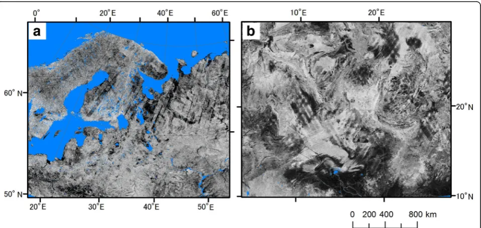
A serious problem in calculating geometric signatures from a fine-resolution DEM is caused by the precision unevenness in different DEM sources and also by the height errors in space-borne DEMs. The differences in spatial resolution or observation instrument (i.e., radar or optical) in source DEMs will cause different patterns of geometric signatures (De Reu et al. 2013; Maynard and Johnson 2014; Ariza-Villaverde et al. 2015). Such unevenness may not be apparent in an image of slope gradient, which is the destination of a primary difference (Evans 1980); however, the noise is more evident in an image uses a concept of secondary difference (e.g., Laplacian filter or curvature) in the calculation process (Guth 2006). Moreover, an image of surface texture (Iwahashi and Pike 2007), which uses a noise detector (median filter) in the calculation process, shows very clear unevenness (Fig. 1).
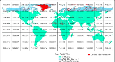
This study used the MERIT DEM that Yamazaki et al. (2017) produced by removing multiple error compo-nents from existing space-borne DEMs. The original MERIT DEM was developed with 3 arc second reso-lution by merging several baseline DEMs (Fig. 2). The data south of 60° N are based on the Shuttle Radar Top-ography Mission 3 arc-second DEM (SRTM3) ver. 2.1 (National Aeronautics and Space Administration; NASA), and the data north of 60° N are based on the
AW3D-30 m DEM ver. 1 (Japan Aerospace Exploration Agency; JAXA). Gaps in these DEMs are filled by the Viewfinder Panoramas DEM (available at http:// www.viewfinderpanoramas.org/dem3.html). Yamazaki et al. (2017) used a 2D-Fourier-transform filter to remove striping and also used ICESat (Ice, Cloud, and land Ele-vation Satellite) laser altimetry data (NASA) to remove absolute bias and vegetation canopy bias. Speckle ran-dom noise was removed by applying an adaptive-scale smoothing filter (Gallant 2011). We resampled the MERIT DEM at 9 arc-second resolution by minimum elevation values for the terrain classification. The mini-mum values were chosen because the MERIT DEM in-cludes buildings that need to be removed as far as possible to bring the values closer to ground data.
In Fig. 3a, the surface texture in another global DEM, GMTED2010 (Danielson and Gesch 2011) shows marked stripe noise (Nelson et al. 2009) origin-ating from the SRTM DEM, whereas the MERIT DEM (Fig. 3b) is almost free from such unevenness. Small areas of the MERIT DEM, which still show unevenness (Fig. 1), were omitted from the terrain classification (Fig. 2). These errors coincided with the
areas where high-quality DEMs (i.e., SRTM or
AW3D) were not available as baseline data for the MERIT DEM. For example, the areas omitted north of 60° N correspond to the observation gap of the AW3D DEM, where the elevations originated from the Viewfinder Panoramas DEM, which has lower effective resolution than AW3D (Fig. 1a, darker areas). The areas omitted in desert regions also
Fig. 1Grayscale images of surface texture from the 280 m MERIT DEM. Unevenness due to DEM source differences is visible:aaround the
correspond to the observation gap of the AW3D DEM, where removal of the stripe noise was not sat-isfactory (Fig. 1b, brighter areas).
The MERIT DEM includes elevations of water bodies on land. Masking of water bodies was mostly achieved using the water bodies in the GlobCover2009 land cover map ver. 2.3 (Bontemps et al. 2013), whose resolution (10 arc-seconds) is close to 9 arc-seconds. The areas at
elevations under 0 m in the MERIT DEM were used as masks for two tiles (50S030 E and 30S150 W in Fig. 2) that show an obvious loss of islands in GlobCover2009.
The DEM resolution is set to 280 m as this corre-sponds to the spatial resolution of a 9 arc-second grid in the mid-latitudes. As Speight (1984) noted, at this resolution, a DEM draws landform patterns rather than landform elements.
Fig. 2Individual tiles and data sources of the MERIT DEM. Each tile covers 20° latitude by 30° longitude. The red areas are omitted in this study
due to unevenness of the DEM (see Fig. 1)
Fig. 3Grayscale images of surface textures in northern Australia from thea250 m GMTED2010 DEM andb280 m MERIT DEM
Calculation of geometric signatures
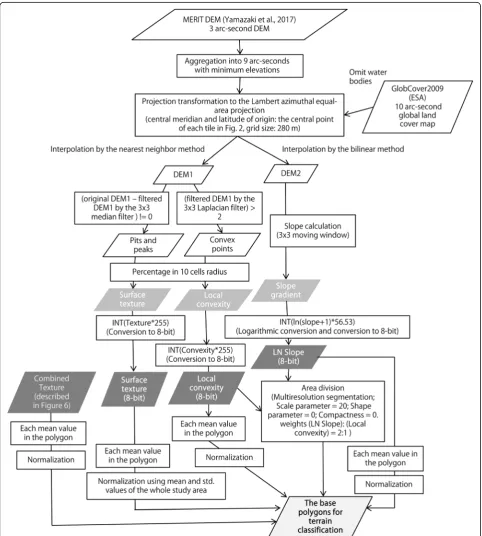
Figure 4 shows the method for generating geometric sig-natures as classifying parameters and area segmentation using the MERIT DEM. First, the MERIT DEM was ag-gregated into 9 arc-seconds as described in the previous
section, a projection transform applied and 280 m DEMs were produced by interpolation with the nearest neigh-bor (DEM1) and the bilinear (DEM2) methods. These two types of DEMs were prepared in order to avoid the noise generated from features of raster image processing
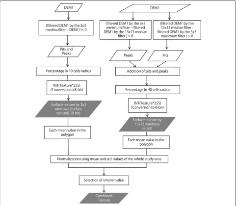
Fig. 4Flowchart for creating the base polygons for terrain classification. The generation of the 280 m DEM, calculation of the geometric
in projection transformation becoming obvious in subse-quent processing. Next, following Iwahashi and Pike (2007), three geometric signatures were calculated: slope gradient (in degrees calculated over 3 × 3 cells), local convexity (spatial density of convex points extracted by the Laplacian filter over 3 × 3 cells), and surface texture (spatial density of pits and peaks extracted by the me-dian filter over 3 × 3 cells). The three geometric signa-tures can be calculated by common image processing software, e.g., ArcGIS Spatial Analyst (ESRI).
Iwahashi (1994) and Iwahashi and Kamiya (1995) introduced the slope gradient to extract mountain slopes from other slopes. In this study, slope gradient was converted logarithmically because, in Iwahashi and Pike (2007), thresholds of classification were defined to be graduated values by a nested-means method, that is, using successively averages of the total slope, the gentler half, the gentlest quarter, and the gentlest quarter-half. This follows a common geomorphological map style in which mountainous steep slopes tend to be lumped together while plains are divided into details. Thresholds of slope gradient for the nested-means method do not decrease linearly like those of surface texture and local convexity, but decrease logarithmically (Iwahashi and Pike 2007). As a consequence, logarithmic converted slope gradient (here-after LN Slope) was used as a classifying parameter in order to replicate the decrease of thresholds in Iwahashi and Pike (2007).
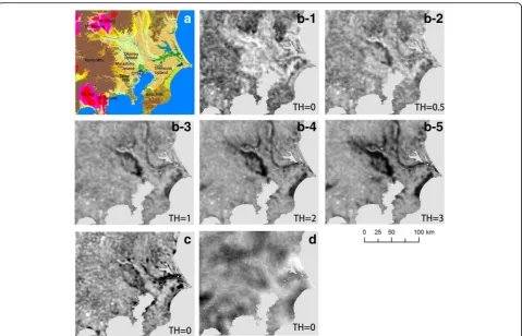
The local convexity tends to be high in terrace sur-faces (Iwahashi and Kamiya 1995). However, the local convexity calculated from different DEMs or using dif-ferent thresholds that separate convex points and others showed very different patterns (Fig. 5, the Kanto District in Japan). The threshold value for extracting convex points used by Iwahashi and Pike (2007) was zero. In this study, we set the threshold value as 2. This value was chosen because we could obtain local convexity im-ages to separate out terrace features and could reduce noise from artificial land as far as possible. Understand-ing of terrace features is important for information on human habitat, ground condition, and flooding in allu-vial topography.
In Japan, surface texture shows relatively low values on debris slopes such as Holocene volcanic slopes and alluvial fans, or high permeability slopes such as weathered granites (Iwahashi and Kamiya 1995). Iwahashi and Pike (2007) showed that the surface tex-ture calculated from the 1-km DEM using 3 × 3 cell windows depicted well the density of mountain ridges and valleys and divided large volcanic cones of Holocene mafic volcanos from older high-texture mountains. The surface texture values calculated from a 50-m DEM showed some correlation with Vs30 data
in Japan (Iwahashi et al. 2010). However, patterns of sur-face texture will change in response to the window size for extracting pits and peaks (Iwahashi and Pike 2007). However, small-scale geomorphological elements, such as cones of small volcanos could be distinguished in 3 × 3 surface texture of the 280 m DEM. A new signature, com-bined texture, was introduced to handle these scale issues. The combined texture was calculated as the minimum value of the normalized 3 × 3 and 13 × 13 surface texture values for each segmented polygon (Fig. 6). Finally, all geometric signatures were normalized to 8 bit to reduce data volume for dealing with processing ability.
Region segmentation
Homogeneous geomorphological elements (Fig. 4) were classified by area segmentation. We used a multi-resolution segmentation method (Baatz and Schäpe 2000) that was implemented in the software eCognition Developer ver.9 (Trimble Inc.). The multi-resolution segmentation method is a technique derived from mov-ing image compression as used in the field of computer vision. The method aggregates neighboring cells that have values closer than a given threshold and then outputs polygons. The advantage is that the method can aggregate cells which include a little unevenness. Drăguţ and Blaschke (2006) used this method for landform clas-sification with 5-, 46-, and 57-m DEMs. Martha et al. (2010) used the method for landslide detection.
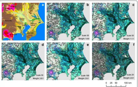
The shapes of polygons output by multi-resolution segmentation change with the choice of geometric signa-tures and their weights. Figure 7 shows some test cases in the Kanto District of Japan. When only LN Slope was used (Fig. 7b) for area segmentation, outlines of terraces and fans were described accurately. However, low ter-races whose cliffs are not clearly defined such as the Omiya Upland (Fig. 7a) could not be outlined clearly. With high-accuracy domestic DEMs, a weight ratio of 1:1:1 for LN Slope:surface texture:local convexity gave good area segmentation (Iwahashi et al. 2015). However, with the 280 m DEM, the weight ratio 1:1:1 gave in-accurate terrace shapes (Fig. 7c). After trial and error, we chose a weight ratio of 2:0:1 for area segmentation using the 280 m DEM. The size of each destination polygon is mainly controlled by the scale parameter (Baatz and Schäpe 2000). We found that a scale parameter of 50 or 100 outputs segments that are too large and omits slightly elevated areas in lowlands (Fig. 7d, e). We finally chose a value of 20, which subdivided homogeneous landforms adequately but not excessively (Fig. 7f ). The shape parameter, which provides a balance between shape and color for segmentation (Kavzoglu and Yildiz 2014), was set to zero following Drăguţ and Eisank (2012). The compactness was also set to zero.
Mean values for each geometric signature (LN slope, surface texture (3 × 3 and 13 × 13), combined texture, and local convexity) within the destination polygons were calculated and stored as representative values. We found much artificial unevenness in residential land. Therefore, we think that the standard deviation should not be used for representative values for the destination polygons, and we used only mean values. After all signa-tures were normalized and the combined texsigna-tures were calculated from the normalized values of 3 × 3 and 13 × 13 surface texture, the base polygon datasets were pre-pared (Fig. 4).
Base classification
There are two kinds of classification method using geometric signatures: image thresholding and data mining. An image thresholding method using LN Slope is conceptually similar to the Iwahashi and Pike (2007) method, if thresholds are configured at equal intervals. The expected advantages are that large data sets can be classified using subdivided data, and classification from mixed DEMs of different data sources may be possible if corrected thresholds are used (Iwahashi et al. 2015). One weakness is that an
inappropriate configuration of thresholds will give nonsensical results. To attach geomorphological meanings to classification results, geometric signatures should be compared with reference materials, and thresholds should be configured after comparison (Iwahashi et al. 2015). However, reference materials are unlikely to be supported globally. Therefore, the image thresholding method is not suitable for global classification.
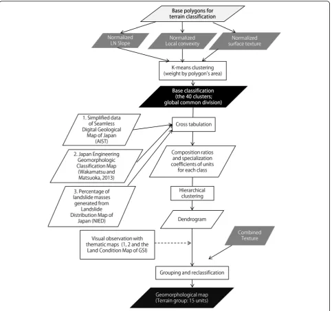
We instead adopted a machine learning method, k -means clustering (MacQueen 1967), for terrain classifi-cation (Fig. 8). The advantages of the clustering are that it can deal with large data and create groups without re-quiring training data. Unsupervised classification exclud-ing subjective judgment will be suitable for comparexclud-ing physical properties of ground with topography. We clas-sified the base polygons created from the 280 m DEM using normalized LN slope, local convexity and surface texture by k-means clustering. The initial number of clusters was set to 40, assuming that the clusters would be reclassified into fewer groups. IBM SPSS Statistics ver.22 was used for k-means clustering and the calcula-tion of all study areas (Fig. 2) converged to 40 clusters at the 682th iteration.
Fig. 5Local convexity in the 280 m DEM from the Kanto District in Japan, calculated with different threshold values (TH) for separating out
Grouping of the clusters and reclassification
The 40 clusters indicate globally unified categories clas-sified by machine learning. In order to identify the type of terrain they represent, we must compare them with existing thematic maps. Moreover, because 40 legends are too numerous for practical use, similar clusters must be merged. We thought that hierarchical clustering, using composition ratios and specialization coefficients of the comparison with thematic maps or data, was ad-equate to understand the similarity of the clusters. It is not necessary for thematic data to be global because it is possible to apply results in representative areas to other areas. Thematic data can be of any form as long as there is a correlation with terrain classification, and grouping of various themes is possible. On the other hand, com-paring the clusters with thematic data that have no
relation to the topography may give meaningless groups. Therefore, we need thematic data that have a wide range, are related to topography, and a map scale that fits the 280 m resolution. Furthermore, as we explained for combined texture, due to the scale of the terrain, the optimal window size for calculating geometric signatures is likely to depend on the region, and additional reclassi-fication may be necessary. In this study, we tested grouping and reclassification using Japanese GIS data in the form of geomorphological maps, geological maps, and landslide distribution maps. Flowcharts of the grouping and reclassification are shown in Fig. 8 and de-scribed in detail below.
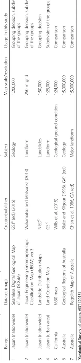
In Japan, the distributions of the 40 clusters were nu-merically compared with existing nationwide geological, geomorphological, and landslide distribution maps (nos.
Fig. 6Flowchart of calculation of the combined texture
1 to 3 in Table 1). Cross tabulation results and graphs are shown in the Additional file 1 with the numbers of clusters.
For the cross tabulations, over 200 types of geologic units from the Seamless Digital Geological Map of Japan (SDGM) (Table 1) were reclassified for statistical con-venience into 14 types according to lithology codes and rock age information in the data attributes. For example,
“Sedimentary rocks” in the geological map was subdi-vided at the age 22 Ma (Middle Miocene), which is known as a boundary between linear and random plots in log–log plots of slope gradient and sedimentary rock age in Japan (Iwahashi et al. 2015). The Miocene is an important era for Japan, as it is the era when the Japan Sea began to open (Otofuji et al. 1985). Subdivision at the Miocene is also useful for imaging boundaries between consolidated and half- or unconsolidated sedi-mentary strata, because sedisedi-mentary rocks younger than the Neogene are often treated as soft rocks in the field of engineering geology in Japan (Japan Society of Civil Engineers 2016). We used full map units (22) of the JEGM (Table 1) for cross tabulation. The JEGM divides populated lowlands and terraces into several groups, but mountains are in one group, except for Holocene
volcanos. Older volcanos are depicted as mountains in the JEGM.
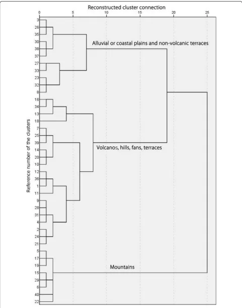
We performed hierarchical clustering using compos-ition ratios and specialization coefficients from the com-parison with geological and geomorphological maps and used percentages of landslide masses to assist grouping. The result shows three meaningful major branches (Fig. 9) compared with the characteristics of each cluster shown in the Additional file 1, i.e., (1) alluvial or coastal plains and non-volcanic terraces, (2) volcanos, hills, fans, and terraces, and (3) mountains. However, in the lower hierarchy, some groups seemed less useful. The result of hierarchical clustering (Fig. 9) was the first priority guide in grouping; however, visual observation of the thematic maps was used to recombine cases where the same mountain masses or terraces were found in different branches. In addition, we used point diagrams of conver-gence values of the clustering (Fig. 10) to check that the clusters within the same group did not differ markedly from each other.
The clusters were grouped into 12 groups. However, the grouping in mountains and hills tended to mix volcanic and non-volcanic mountains that could easily be distinguished by visual investigation with geological
Fig. 7The area segmentations using different weights and scale parameters on the Kanto District in Japan. TheaJEGM geomorphological map
maps. Some, but not all, could be divided by surface texture calculated from a 1-km resolution DEM (Iwahashi and Pike 2007); therefore, the mixing was caused by the use of smaller sized windows for surface texture. We used the combined texture as an additional threshold parameter. Thresholds were decided by visual observation of the image of combined texture compared with the landform elements of JGEM and the 1:25,000 Land Condition Map of the Geospatial Information Authority of Japan (no. 4 in Table 1). The latter are geomorphological maps of urban plains and their sur-roundings, which have been published from the 1960s. The extra three groups found by this reclassification of mountains and hills gave a total of 15 definitive terrain groups. Table 2 gives quantitative descriptions of the 15 terrain groups.
Results
Cross tabulations with geological and geomorphological data
The terrain classification using DEM objectively distin-guishes homogeneous slopes. In this study, we grouped slopes of similar properties by hierarchical clustering using Japanese thematic maps and reclassified mountains and hills by the combined texture. The final 15 groups were cross tabulated and visually compared with Japanese the-matic maps again. Moreover, we also conducted the same analysis for overseas areas where public data can be ob-tained. We chose three scopes: an area that lies in a young orogenic belt like Japan (California), an area totally differ-ent from Japan in geological and climate settings
Fig. 8Flowchart of terrain classification used to generate a geomorphological map
Fig. 9(See legend on next page.)
(See figure on previous page.)
Fig. 9Dendrogram of the 40 clusters obtained by hierarchical clustering in Japan. This figure shows a dendrogram calculated by the Ward
method, using composition ratios and specialization coefficients of the comparison with JEGM and SDGM, and percentages of landslide masses (Table 1). Numbers in the left column of the graph are the reference numbers of the 40 clusters in the Additional file 1. The text in this graph shows typical landforms for the three branches
(Australia), and glacier regions that are rare in Japan but very important for landform formation in high-latitude areas. These analyses were important in order to construct the final legend.
Comparisons with the geological and geomorphological maps of Japan
We compared the statistics of the 15 groups and geo-morphological and lithological data (Table 3). Table 3 lists not only composition ratios (CR) but also particularly large values (> two times) of specialization coefficients (SC) were described in Table 3, because map scales differ substantially (Table 1).SCdescribes the level of concentra-tion of a certain map unit in the clusters. SC exceeding one indicates concentration of the distribution. This trend is more pronounced with largerSCvalues.
The result of grouping using Japanese geomorphological and geological data (SDGM and JEGM) generally implied the following. Groups 1 and 2 were bedrock mountains. In group 3, there were more sediments that were probably talus or dissected terraces, and the group indicated middle-relief mountains. Therefore, group 3 was hills. Among groups 1 to 3 (i.e., bedrock mountains and hills), there was a difference in major rock types in the sub-categories“a”and“b”as intended. Sub-category a seemed to be hard rocks, and b included debris and high-permeability rocks. On the other hand, Table 2 shows the difference between b of bedrock mountains and hills. Sub-category b in bedrock mountains was smooth on both large and small scales; however, b in hills was rough on the large scale. Groups 4 and 5 were highland slopes that
were steep but very smooth (Table 2), and they were closely related to Holocene mafic volcanos and their sur-roundings. Groups 6 to 12 were terraces, fans, and plains formed by unconsolidated strata. Their slope gradients were small and their average surface texture gradually de-creased (Table 2). Groups 6 and 8 coincided closely with the Japanese major terrace type, i.e., terraces covered with volcanic ash soils (Wakamatsu and Matsuoka 2013). Group 7 was also terraces in a broad sense; however, spe-cifically, it was rather fans or valley bottoms that were mainly distributed in shallow valleys in terraces. Group 9 mainly represented Japanese major alluvial fans that were formed by sands and gravels. Groups 10 to 12 covered al-luvial plains, coastal plains, and their surroundings. Group 10 was plains at the foot of mountains. Groups 11 and 12, especially group 12, were very gentle slopes and widely distributed in muddy and silty plains.
The categories with low CR (< 5%) that were not de-scribed in Table 3 were mainly as follows. Plutonic rocks (Middle Miocene to Holocene), ultramafic rocks, and felsic intrusive rocks had high SC values in group 1a. HighSC values also appeared in groups 3b, 6, and 9 for Holocene tephra; groups 5, 6, and 7 for rocky strath ter-races; groups 8, 10, and 11 for sand bars and dunes in coastal plains; and groups 6, 8, and 10 for filled land. Additional visual observation revealed that distinctive terrain with long slopes, such as caldera escarpments (e.g., Aso caldera, Kumamoto Prefecture, Kyushu), fault-block mountains (e.g., Yourou Mts., Gifu Prefecture, Honshu), and inselberg (e.g., Mt. Tsukuba, Ibaraki Prefecture, Honshu) were classified as group 1b.
Table 2Quantitative values of the terrain groups, calculated globally
Terrain group
Cluster reference numbers (see Additional file1for Japanese conditions)
Average of slope gradient Average of surface texture Average of local convexity Threshold of combined texture
Average of combined texture
Degrees Z scorea % Z score % Z score
1a 6, 15, 22, 40 14.8 2.25 70 0.77 43 0.85 > 0.41 0.72
1b 14.9 2.25 63 0.42 42 0.75 ≦0.41 0.15
2a 5, 17, 19, 29 7.8 1.54 73 0.94 41 0.62 > 0.15 0.69
2b 6.5 1.34 68 0.65 38 0.43 ≦0.15 −0.20
3a 4, 7, 10, 14, 20, 24, 25, 31, 39 2.8 0.50 71 0.79 40 0.55 > 0.1 0.51
3b 1.7 0.10 71 0.83 39 0.46 ≦0.1 −0.43
4 18 7.5 1.49 55 −0.03 45 0.94 −0.08
5 16, 34 2.7 0.49 57 0.06 44 0.85 −0.03
6 2, 21, 28, 37, 38 0.8 −0.38 67 0.63 40 0.55 −0.06
7 9 1.3 −0.10 61 0.28 37 0.29 0.10
8 3, 26, 30 0.4 −0.72 55 −0.05 34 0.08 −0.46
9 1, 11, 12, 13, 36 0.9 −0.35 47 −0.46 35 0.18 −0.58
10 35 0.3 −0.82 42 −0.72 25 −0.62 −0.91
11 27, 32, 33 0.2 −0.93 30 −1.37 16 −1.38 −1.45
12 8, 23 0.1 −1.04 14 −2.20 3 −2.45 −2.20
a
1 Normalized value using global average and standard deviation
Table 3CRaandSCbof geomorphological and geological units for each terrain group in Japan
Terrain group
Landform element of JEGM Geological unit of SDGM
1a Mountain (84%), volcanoc(8%), others (8%) Accretionary complex (30%), mafic volcanic rocks (Jurassic to Pleistocene) (20%), plutonic rocks (Silurian to Middle Miocene) (13%), felsic volcanic rocks (9%),metamorphic rocks(9%) (× 2.3), others (19%)
1b Mountain (53%),volcano(32%)(× 7.0), volcanic footslope (9%), others (6%)
Mafic volcanic rocks (Jurassic to Pleistocene)(39%) (× 3.1), accretionary complex (13%), Plutonic rocks (Silurian to
Middle Miocene) (10%), sediments (8%), felsic volcanic rocks (7%), pyroclastic flow deposits (6%)
2a Mountain (79%), others (21%) Accretionary complex (25%), mafic volcanic rocks (Jurassic to Pleistocene) (18%), plutonic rocks (Silurian to Middle Miocene) (13%), sediments (13%), felsic volcanic rocks (12%), sedimentary rocks (Silurian to Middle Miocene) (7%), metamorphic rocks (6%), others (6%)
2b Mountain (70%), hill (9%), volcano (7%), others (14%) Sediments (23%), accretionary complex (22%), mafic volcanic rocks (Jurassic to Pleistocene) (17%),sedimentary rocks (Silurian to Middle Miocene)(13%) (× 2.3), felsic volcanic rocks (9%), plutonic rocks (6%), others (10%)
3a Mountain (36%), hill (23%), gravelly terrace (11%),valley bottom lowland(10%) (× 2.0), volcanic footslope (5%), others (15%)
Sediments (38%), accretionary complex (13%), Plutonic rocks (Silurian to Middle Miocene) (12%), mafic volcanic rocks (Jurassic to Pleistocene) (9%), pyroclastic flow deposits (8%), sedimentary rocks (Silurian to Middle Miocene) (7%), felsic volcanic rocks (7%), others (6%)
3b Hill(32%) (× 3.1), mountain (20%), gravelly terrace (10%), volcanic footslope (9%), valley bottom lowland (8%), terrace covered with volcanic ash soil (6%),volcanic hill(6%) (× 2.4), others (9%)
Sediments (54%),pyroclastic flow deposits(13%) (× 2.3), accretionary complex (7%), sedimentary rocks (Silurian to Middle Miocene) (7%), mafic volcanic rocks (Jurassic to Pleistocene) (5%), others (14%)
4 Volcano(55%) (× 12.5),volcanic footslope(36%) (× 7.7), others (9%) Mafic volcanic rocks (Holocene)(47%) (× 84.3),volcanic debris (Miocene to Holocene)(21%) (× 12.6), mafic volcanic rocks (Jurassic to Pleistocene) (16%), pyroclastic flow deposits (8%), others (8%)
5 Volcanic footslope(60%) (× 12.8), gravelly terrace (10%),terrace covered with volcanic ash soil(9%) (× 2.3), volcano (6%), others (15%)
Sediments (35%),volcanic debris (Miocene to Holocene)(23%) (× 13.9),pyroclastic flow deposits(18%) (× 3.1),mafic volcanic rocks (Holocene)(14%) (× 25.8), mafic volcanic rocks (Jurassic to Pleistocene) (7%), others (3%)
6 Terrace covered with volcanic ash soil(19%) (× 4.8),gravelly terrace
(16%) (× 2.4),valley bottom lowland(14%) (× 3.0), hill (12%), volcanic footslope (7%),back marsh(7%) (× 2.5), alluvial fan (7%) (× 2.3),delta and coastal lowland(5%) (× 3.1), others (13%)
Sediments(79%) (× 2.3), pyroclastic flow deposits (8%), others (13%)
7 Gravelly terrace(29%) (× 4.2),terrace covered with volcanic ash soil
(14%) (× 3.5), hill (13%),alluvial fan(12%) (× 4.3),valley bottom lowland(10%) (× 2.2), volcanic footslope (8%), others (14%)
Sediments(81%) (× 2.4), pyroclastic flow deposits (5%), others (14%)
8 Terrace covered with volcanic ash soil(19%) (× 4.8),alluvial fan(16%) (× 5.7),gravelly terrace(15%) (× 2.2),back marsh(14%) (× 5.2),delta and coastal lowland(8%) (× 4.7), others (28%)
Sediments(95%) (× 2.8), others (5%)
9 Alluvial fan(30%) (× 10.5),gravelly terrace(30%) (× 4.4),terrace covered with volcanic ash soil(16%) (× 4.1),volcanic footslope
(10%) (× 2.1), others (14%)
Sediments(86%) (× 2.5), pyroclastic flow deposits (5%), others (9%)
10 Back marsh(28%) (× 9.9),alluvial fan(22%) (× 7.5),delta and coastal lowland(14%) (× 8.3), gravelly terrace (8%),natural levee(7%) (× 11.2), others (21%)
Sediments(99%) (× 2.9), others (1%)
11 Back marsh(36%) (× 13.1),delta and coastal lowland(18%) (× 10.9),
alluvial fan(12%) (× 4.3),natural levee(11%) (× 17.1),reclaimed land
(6%) (× 13.3), others (17%)
Sediments(100%) (× 2.9)
12 Back marsh(56%) (× 20.0),delta and coastal lowland(21%) (× 13.0),
natural levee(14%) (× 21.0),reclaimed land(7%) (× 14.7), others (2%)
Sediments(100%) (× 2.9)
Legends withCRof 5% or more are shown. Clusters withSCover × 2.0 are shown in bold text and the factors are in parentheses
a
Composition ratio
b
specialization coefficient
c
Comparisons with geohazard data and densely inhabited district data in Japan
In Japan, the Ministry of Land, Infrastructure and Transport (MLIT) has published some national statistics as GIS data,
“National Land Numerical Information”. Wakamatsu (2011) collected spatial data of historic (745 A.D. to 2008 A.D.) liquefaction in Japan. We analyzed the relationship between the subjects concerning such land conditions and each ter-rain group. Table 4 shows CR andSCof terrain group vs. densely inhabited districts (DID), sediment disaster hazard areas, and historic liquefaction. The sediment disaster hazard areas, which describe dangerous zones susceptible to col-lapse, mud or debris flows, and landslides, are not specified in regions with no or few downstream habitations. There-fore, we calculated corrected specialization coefficients (CSC) in Table 4 by using distribution percentages of the DID areas (CSC:SC/CRin the DID areas for each group).
The GIS data of historic liquefactions (Wakamatsu 2011) describe newer liquefactions after the World War II that can be delineated on maps or aerial photographs as polygons and describe the first liquefaction that ap-pears in Japanese historical documents (745 A.D.) to the last liquefaction within the data collection period (2008 A.D.) as point data of the centers of liquefied areas. The point data include 3717 liquefaction sites, but many of these are near seashores and overlap with the water body
of the GlobCover 2009. Therefore, 2914 of the point data were used in the analysis.
The DID areas in Japan were remarkably concentrated in groups 6 to 12. Although the highestSCvalue was in group 8 that was mainly low terraces, the distributions of errors caused by reclaimed land around coastal areas may have raised SC. The liquefaction sites in polygon form were mainly distributed in groups 11 and 12, which were very gentle slopes. However, point data of liquefac-tion sites were concentrated on steeper slopes which correspond to terrains, alluvial fans, and hills. According to individual investigation of those sites, hilly cases were divided into three types: banking on residential areas, exceedingly strong earthquakes which occurred in hills of sedimentary rocks (e.g., the Chuetsu Earthquake on 23 October 2004), and insufficient DEM resolution that missed narrow plains along valleys or coastlines.
The zones susceptible to collapse in Japan and officially considered dangerous are defined by the MLIT as steep slopes (over 30° and 5 m high) and their surrounding habi-tats. These zones were concentrated not only in the groups representative of bedrock mountains (groups 1 and 2) but also in highland slopes that were thought to be formed by debris or high permeability rocks (groups 4 and 5), espe-cially in group 4.CSCvalues were also very high in the case of the officially defined zones of landslides and debris flow.
Table 4CRa,SCb, andCSCcof DIDdand geohazards for each terrain group in Japan
All Japan
DID Dangerous zones for the sediment disaster hazard area Historic liquefaction
Collapse Landslide Debris flow Center point (745 A.D. to 2008 A.D.)
Polygon (after WW2)
Terrain group CR(%) CR(%) SC CR(%) CSC CR(%) CSC CR(%) CSC CR(%) SC CR(%) SC
1a 13.2 0.1 0.0 5.3 5.7 11.0 11.9 3.9 4.3 0.0 0.0 0.0 0.0
1b 2.6 0.1 0.0 1.0 7.3 2.1 16.0 1.5 11.0 0.0 0.0 0.0 0.0
2a 31.9 1.0 0.0 32.4 1.0 43.5 1.3 33.3 1.0 0.1 0.0 0.1 0.0
2b 4.0 0.5 0.1 3.4 1.9 7.7 4.2 4.5 2.5 0.0 0.0 0.0 0.0
3a 20.6 8.2 0.4 37.9 0.2 24.6 0.1 40.1 0.2 4.1 0.2 1.1 0.1
3b 9.6 7.7 0.8 12.9 0.2 10.0 0.1 9.7 0.1 9.2 1.0 4.0 0.4
4 0.3 0.0 0.0 0.1 44.0 0.1 60.8 1.0 402.9 0.0 0.0 0.0 0.0
5 0.6 0.5 0.8 0.5 1.7 0.2 0.6 2.5 8.5 0.0 0.1 0.0 0.0
6 6.5 23.0 3.5 4.7 0.0 0.6 0.0 1.7 0.0 17.6 2.7 9.0 1.4
7 1.2 3.9 3.3 0.9 0.2 0.2 0.0 1.4 0.3 1.3 1.1 0.4 0.3
8 4.6 34.3 7.5 0.6 0.0 0.1 0.0 0.2 0.0 34.4 7.5 29.9 6.6
9 1.1 3.1 2.9 0.2 0.1 0.1 0.0 0.2 0.1 0.2 0.2 0.7 0.6
10 1.4 6.3 4.6 0.1 0.0 0.0 0.0 0.0 0.0 29.0 21.1 12.8 9.3
11 2.2 9.5 4.3 0.0 0.0 0.0 0.0 0.0 0.0 3.7 1.7 34.9 15.8
12 0.4 1.9 5.1 0.0 0.0 0.0 0.0 0.0 0.0 0.3 0.7 7.2 19.0
a
Composition ratio
b
specialization coefficient
c
specialization coefficient corrected by the composition ratio of units in the DID area of terrain groups
d
Densely inhabited districts
In these cases, smooth steep slopes (groups 1b, 2b, and 4) show higherCSCvalues.
Comparison with theVs30 data in Japan
The ground Vs30, which is observed or estimated by borehole data, is a predictor of earthquake ground motion amplification. We compared the calculated
Vs30 based on published shear-wave velocity profile data in Japan (Strong-motion Seismograph Networks, K-NET and KIK-net by NIED; http://www.kyoshin.bo-sai.go.jp) with the terrain classification (Fig. 11). In extremely steep slope areas (Additional file 1) like groups 1a and 1b, there is a possibility that Vs30 values were measured on narrow valley floors that are not described by the 280 m DEM.
The box plot in Fig. 11 shows relatively low medians for smooth slopes (1b, 2b, and 3b) in mountains and
hills. However, among intermediate landforms, thought to be formed by half- or unconsolidated strata, fan-predominant slopes (groups 7 and 9) showed higher
Vs30 values than terrace-predominant slopes (groups 6 and 8) that were usually rougher than fans. In plains, (groups 10 to 12), Vs30 values decreased along with slope gradients.
Comparisons with data from California, Australia, and glacier regions
Cross tabulations were performed with geological or lithological maps of California and Australia in order to investigate if the Japanese grouping of the clusters was also meaningful for other regions (Table 5). California lies on a young orogenic belt like Japan, but there are no Holocene volcanos and the climate is drier than in Japan. Australia mostly lies on very dried shields and
Table 5 CR a and SC b of geomorphological and geologic al units for each terrain group in California and Australia Terrai n group Cali fornia, litholog ical unit of Wi lls et al. ( 2015 ) Australia, ge ological unit recla ssified c from Blake and Kilgour ( 1998 ) Aus tralia, major landform unit of Chan et al. ( 1986 ) 1a Cr ystalline rock s (61%) (×2 .1), Fra ncisca n compl ex rock s (17%) (×2.7), Te rtiary volcan ic unit s (8%) , Tert iary sandsto ne units (6%) , others (8%) Sedime ntary ro cks (51%), granites (19%), fe lsic vol canics (8%) (×5 .8), m afic intrus ives (6% ) (×9.1), Cenozo ic maf ic volcanic s (6%) (×4 .1), metamorp hic s (6%) , othe rs (4%) Moun tains (59%) (×1 0.1), plate au (15%), hills (12%) , low hill s (7%) 1b Cr ystalline rock s (59%) (×2 .0), Tert iary volcanic units (19%), Tert iary sandst one unit s (5%) , othe rs (17%) Sedime ntary ro cks (49%), grani tes (29%) (×2 .9), metamorp hic s (5%) , othe rs (17%) Hills (35%) (×3.2 ), m ountains (34%) (×5 .8), low hill s (7%) 2a Cry stalline rocks (45%), Tertiary sandston e units (14%), Fra nciscan com plex ro cks (13%) (×2 .0), Te rtiary volcan ic unit s (9%) , Tert iary shal e an d silts tone units (7% ), oth ers (12%) Sedime ntary ro cks (58%), granites (16%), fe lsic vol canics (6%) (×4 .4), Cenoz oic mafic volcanics (6%) (×4 .1), others (14%) Moun tains (45%) (×7 .7), hill s (21%), low hill s (11%) 2b Cry stalline rocks (36%), Tertiary volc anic units (15%) , Tertiary sandsto ne un its (14%), Holocene alluvium (steep slopes ) (12%), Cre taceous sa ndston e (6% ) (×2.8 ), Tert iary shale an d silts tone units (6% ), othe rs (11%) Sedime ntary ro cks (66%), granites (12%), me tamorphics (7%), others (15%) Hills (24%) (×2.2 ), m ountains (23%) (×4 .0), pla teau (17%) , low hill s (12%), rises (7%) 3a Cry stalline rocks (32%), Tertiary volc anic units (18%) , Tertiary sandsto ne un its (11%), Holocene alluvium (steep slopes ) (9%), Franciscan compl ex un its (7%) , Tert iary shal e an d siltston e units (6% ), Pleis tocene all uvium (6% ), Pleis tocene -Plioc ene alluvial deposi ts (5%) , others (6%) Sedime ntary ro cks (55%), granites (17%), m afic volcan ics (6%) (×2 .2), fe lsic vol canics (6%) (×4.2), others (16%) Hills (30%) (×2.8 ), low hills (23%) (×2 .1), m ountains (22%) (×3 .9), pla teau (13%) 3b H oloce ne all uvium (stee p slop es) (22%) (×2.1 ), crys talline rocks (16%) , Te rtiary volcan ic unit s (14%), Tertiary sandston e units (14%) , Pleist ocene all uvium (12%) , Pleis tocene – Plioc ene alluv ial depos its (7% ) (×2.9), Tertiary shal e an d silts tone units (7% ), othe rs (8% ) Sedime ntary ro cks (62%), Cenozoi c rego lith (10%) , granite s (10%), me tamorphics (6%) , othe rs (12%) Hills (23%) (×2.1 ), low hills (20%) , mou ntain s (14%) (×2 .4), pla teau (13%) , rises (9% ), eros ional pla in (6% ) 4 Ter tiary vol canic units (39%) (×3.5 ), crys talline rocks (25%) , Holoc ene all uvium (s teep slopes) (18%), Pleist ocen e alluvium (8%) , others (10%) Sedime ntary ro cks (58%), mafic volcan ics (13%) (×4.8 ), Ceno zoic mafic vol canics (8% ) (×5.2), meta morph ics (6%), Cenozoi c rego lith (5%), others (10%) Hills (37%) (×3.4 ), low hills (22%) (×2 .0), m ountains (20%) (×3 .5), lav a plain (7%) (×1 0.3), plate au (6%) 5 H oloce ne all uvium (stee p slop es) (44%) (×4.3 ), Pleis tocene alluvium (19%) , crys talline rocks (15%) , Tert iary vo lcanic units (13%) , othe rs (9%) Sedime ntary ro cks (65%), Cenozoi c rego lith (15%) , Ceno zoic mafic vol canics (7% ) (×5.0), othe rs (13%) Low hills (30%) (×2 .8), hills (22%) (×2.1 ), coa stal dune s (7%) (×1 4.8), dunef ield (7% ), lava pla in (6% ) (×9.3), mou ntains (6%) 6 Ter tiary sand stone uni ts (19%) (×2.3), Tertiary volc anic units (19%) , Pleis tocene all uvium (18%) , Holoc ene alluvium (steep slopes ) (13%), crys talli ne rocks (10%), Ho locene all uvium (mo derate slopes) (8% ), Pl eistoc ene – Plioce ne all uvial dep osits (7%) (×3 .0), othe rs (6% ) Sedime ntary ro cks (47%), Cenozoi c rego lith (20%) , granite s (13%), me tamorphics (6%) , mafic vol canics (6%) (×2 .1), othe rs (8% ) Hills (25%) (×2.3 ), low hills (18%) , mou ntain s (11%) , plateau (10%), ris es (9%) , dunef ield (8%) , sand plain (6%) , erosion al plain (5%) 7 Ter tiary vol canic units (24%) (×2.1 ), Ple istoce ne all uvium (21%) (×2.0), H oloce ne all uvium (steep slopes) (21%) (×2 .0), crys talli ne rocks (10%), Te rtiary sandstone units (8% ), Pleis tocene -Pliocene alluvial deposi ts (5% ), oth ers (11%) Sedime ntary ro cks (57%), Cenozoi c rego lith (15%) , granite s (11%), me tamorphics (6%) , othe rs (11%) Hills (23%) (×2.1 ), low hills (17%) , pla teau (14%), dune field (12%) , rises (10%) , mou ntains (9%) , eros ional pla in (6% ) 8 H oloce ne all uvium (mode rate slopes ) (28%) (×4 .2), Pl eistoc ene alluvium (23%) (×2.2), tertiary volc anic units (21%) , Holoc ene alluvium (very low slop es) (8% ), tert iary sandstone units (8% ), Holoc ene alluvium (stee p slop es) (6% ), othe rs (6% ) Cenozoi c rego lith (42%), sedim entary rocks (36%), granite s (8%) , meta morph ics (5% ), othe rs (9% ) Dun efield (23%) (×2.2 ), sand plain (13%), pla teau (12%) , erosion al plain (11%), rises (9%) , low hills (8% ), hill s (8%) , deposi tiona l plain (6%) 9 H oloce ne all uvium (mode rate slopes ) (34%) (×5 .1), H olocene all uvium (st eep slopes) (32%) (×3.1), Pleis tocene alluv ium (21%) (×2.0), Tert iary vo lcanic units (5%), others (8%) Sedime ntary ro cks (36%), Cenozoi c rego lith (32%) , granite s (18%), me tamorphics (6%) , othe rs (8%) Plat eau (23%) (×2 .1), eros ional pla in (16%), dune field (14%) , sand pla in (10%), low hills (9% ), ris es (8%), hills (6% ), de positio nal pla in (6% )
platforms. In many regions, Japan and Australia are to-tally different regarding climate and geological settings. The geological map of Australia (Blake and Kilgour 1998) has over 200 categories, so geologic units were ag-gregated to 15 categories, considering rock age and lith-ology. We used all 26 categories of the regolith terrain map of Australia (Chan et al. 1986) as geomorphological data. The regolith terrain map used in this study is at a scale of 1:5,000,000 and valley plains were not repre-sented in sufficient detail. For California, we used the
Vs30 map of Wills et al. (2015), which aggregated and supplemented the geological map of California with esti-mated seismic amplification.
In a general division between hard rocks and uncon-solidated strata, Tables 3 and 5 show that Japan and California are alike in that mountains are formed by bedrocks and plains are formed by sediments. Although there are no Holocene volcanos in California, there are some characteristics in common with Japan; in group 4, volcanic rocks were predominant, and in groups 3 and 5, steep Holocene alluvium that may coincide with talus was predominant. Similar to Japan, groups 6 to 8 were mainly depositional terrains in California. Group 9 was predominant in sandy and gravelly alluvial fans in Japan, but in dry areas of California such as the Basin and Range provinces, it was often distributed in pediplains and bajada that were formed under a dry climate. Although groups 11 and 12 were mainly formed by very low Holocene alluvium like in Japan, Pleistocene allu-vium was also distributed and gave some terrain age that was older than that in Japan.
In the case of Australia, groups 1 and 2 were composed of bedrocks, and gentler slopes included more unconsoli-dated strata like in Japan. However, lithological character-istics for each group were evidently different from Japan and California. All terrain groups in Australia included a similar pair of sedimentary rocks and granites, even in plains. It is well known that bedrocks form erosional plains in Australia after very long-term erosion on the stable continent. This was consistent with our data that erosional plains were predominant in groups 10 to 12, and
SC values of pediplains were slightly high in groups 10 and 11. Australian mountains showed different predomin-ant lithology in the subcategories a and b, but Cenozoic mafic volcanics appeared in a, though similar lithology often appeared in b in Japan. On the other hand, there were some common points with Japan, that is, alluvial plains, flood plains, and flood outs were predominant in group 12, and lava plains were predominant in groups 4 and 5. It was quite strange that “hills” appeared in all groups in Australia. We thought that there was a possibil-ity that many valley plains were omitted because of the map scale (1:5,000,000; Table 1). Plateaus also appeared in many groups from mountains to plains. In Japan, plateaus
formed by bedrock table mountains as in Australia are rare except for volcanics, and most of the “plateaus” are actually diluvial uplands. In Australia, the difference be-tween plateaus distributed in different groups probably depended on the proportions between tablelands and plat-eau edges observed in the 280 m grid. Platplat-eaus were espe-cially predominant in group 9, where fan-shape slopes were distributed in Japan and California. The categories with low CR(< 5%) that were not described in Table 5 were mainly as follows. Coastal dunes showed high SC values in group 5, and glacial features showed the highest
SCvalue in group 1b and highSCvalues in groups 3a, 1a, and 2a.
We noted glaciated mountains that were rare in Japan, California, and Australia. Those in the Canadian Rockies and Alps were visually observed using glacier inventory maps (RGI Consortium 2017). The results showed that glacier areas were mainly distributed in groups 1a and 1b, and group 1b covered the areas surrounding glaciers.
Classification map and estimated legends
The final legends for the terrain groups are given in Fig. 12. The descriptions in Fig. 12 were obtained by the methods described in the previous sections. Although this legend mainly shows the groups constructed from Japanese geo-logical and geomorphogeo-logical information, the main cat-egories that divided the terrain into (1) bedrock mountains; (2) hills; (3) large highland slopes; (4) plateaus, terraces, and large lowland slopes; and (5) plains are probably applicable globally. We noted the landform patterns not only in Japan but also in California and Australia for arid landforms. Figure 13 shows a thumbnail image of global polygon data classified according to the terrain groups in Fig. 12. The classification is obviously improved from Iwahashi and Pike (2007) in representations of terrace shapes (Fig. 14) and landform elements smaller than 1 km (Fig. 15).
Although the global terrain was classified into groups that were categorized using Japanese thematic data, dis-tinct topographies of various locations were also well depicted. For example, terrain classification data from Krasnoyarsk (Fig. 16) clearly depicted lava of Siberian Traps (Svensen et al. 2010). Terrain classification data for central New Zealand (Fig. 17) and the Cameroon line (Fig. 18) also depict well of volcanoes and other moun-tains in addition to alluvial or coastal lowlands.
In contrast, metropolitan areas, especially in coastal areas, are misclassified as terrace-like groups, i.e., groups 8, 10, and 6 (e.g. Tokyo Gulf Coast in Fig. 14). This is probably caused by DSM (digital surface model) charac-teristics of the 280 m DEM rather than the influence of artificial slopes. Moreover, limits in the specification of the geometric signatures may still prevent the detection of slight rises in gentle plains. For example, the terrain of the Central
Fig. 12Legend of the terrain classification
Plain of Thailand (Fig. 19) is classified poorly compared with a manual classification map (Ohkura et al. 1989).
Discussion
Validity of the geometric signatures
It is well known that the values and spatial patterns of geometric signatures differ according to the accuracy and resolution of DEMs (Zhang and Montgomery 1994; Armstrong and Martz 2003; Deng et al. 2007; Wu et al. 2007; Maynard and Johnson 2014). Unevenness of DEMs will lead to less accurate classification of topog-raphy. For this reason, we used the MERIT DEM for ter-rain classification.
The three-part geometric signatures adopted in this study generally gave satisfactory results for terrain classi-fication. The new parameter, the combined texture, may help depict both small-scale and large-scale smooth
slopes. In the case of plains, the limit of the description of geometric signatures was mainly caused by insuffi-cient DEM resolution. This problem should be solvable in the future using higher resolution DEMs. For example, the MERIT DEM is originally 3 arc-seconds resolution. However, high-resolution DEMs may create considerable problems in terrain classification owing to the appearance of artificial smoothing or cutting of land. An additional method from using the original elevations, instead of their derivatives, will be needed for more de-tailed classification of plains because the derivatives may emphasize artificial errors (Erskine et al. 2007).
Tuning of geometric signatures can give very different descriptions, for example, patterns of local convexity changed dramatically with threshold values in calculat-ing convex points (Fig. 7). In this study, we set thresh-olds of local convexity so as to extract terraces.
Fig. 14Comparison of terrain classification images of the Kanto District and its surroundings.aJEGM (Wakamatsu and Matsuoka 2013).bResults
of this study, using the 280 m DEM.cIwahashi and Pike (2007), using a 1 km DEM
However, different threshold values might possibly out-put better classification results for other purposes or other DEMs.
Considering the calculation cost and expected degree of improvement, and the ability to add another param-eter later because the threshold processing had been performed using combined texture, we did not think that the addition of another geometric signature was necessary for clustering. However, the mixture of deposi-tional landforms and erosional landforms (e.g., fans and
pediplains in group 9) seems to be a major problem in continental regions where both alluvial landforms and arid landforms exist.
Validity of the region segmentation and clustering
In terms of region segmentation, we did not think that many parameters were necessary for drawing boundary lines of landforms, and the results of object segmentation using LN slope and local convexity effectively separated the range of similar landform
Fig. 15Comparison of the terrain classification images of the Rub’al khali.aResults from of this study, using the 280 m DEM.bIwahashi and
Fig. 16Shaded terrain classification image in the Krasnoyarsk region (Russia)
patterns as considered in the section “Region segmen-tation”. A scale parameter of 20 seems to be rather small on continents, but is mostly adequate (or rather too large) for Japan where various micro geomorpho-logical elements are distributed. Smaller values for the scale parameter will create a large volume of polygon data and will make it difficult to use the data. We thought 20 was adequate globally for the scale param-eter. The polygon-based format helps to edit or merge terrain classification data easily.
The 40 clusters obtained by k-means clustering were globally common divisions, because the cluster-ing was done uscluster-ing all polygon attributes. Although the final number of clusters is arbitrary in k-means clustering, the calculation cost tends to increase as the number of clusters increases, and the calculation does not converge with too many clusters. Moreover, too many clusters will make data usage rather difficult. Considering this, we decided on the final number of clusters as 40.
Validity of the grouping and reclassification
In the hierarchical clustering in Japan, bedrock moun-tains constituted clearly separate branches from other
terrain types. The difference of geological and geomor-phological characteristics between bedrock mountains and others was relatively clear. Among the bedrock mountains and hills, we distinguished two types of slopes, sub-categories a and b. Suzuki (2002) gives a schematic diagram showing the relationship between the relief and drainage density, and the strength and perme-ability of bedrock. The diagram shows that hard rocks form high-relief mountains, soft rocks form low-relief mountains (or hills), low permeability rocks form straight slopes, and high permeability rocks form convex slopes. Surface texture (i.e., the density of pits and peaks that coincide with valley lines and ridges in the 280 m grid scale) is related to drainage density, and local con-vexity is related to the concon-vexity of slopes. In sub-category b, which had a lower drainage density than a, highly permeable types of rocks such as old mafic volcanic rocks and sedimentary rocks were more pre-dominant than very hard rocks such as accretionary complex and metamorphic rocks. This was consistent with the findings of Suzuki (2002) and indicated that it may be permeability that separates a and b of mountains and hills in Japan. Indeed, groups 1b and 2b were pre-dominant in crushed or high permeability rocks such as
Fig. 18Shaded terrain classification image of the Cameroon line and Niger delta
weathered lava and old sedimentary rocks in Japan and showed lowerVs30 values (Fig. 11). Groups 4 and 5 were unique groups; they were clearly predominant in un-dissected mafic volcanos and volcanic footslopes in Japan and showed very high correlation with the sedi-ment disaster hazard area (Table 4). Not exactly the same, but similar lithologic trends of groups 4 and 5 could be observed even in California and Australia. The relationship between lithology and landforms in moun-tains has been explored in various ways, e.g., the relationship between slope materials and slope surface (Kenter 1990) and rock control (Yatsu 1966). Moreover, lithology and rock hardness have broad study fields in engineering geology and have been widely discussed for rock mass classification since Terzaghi (1946). Some rock mass classifications focus on classification of lith-ology (e.g., Marinos and Hoek 2000). Thus, especially under the same climatic and geologic province, search-ing for similar topography in mountains and hills may help to at least grasp some common points of physical properties of the ground.
Intermediate landforms formed by half- or unconsoli-dated strata were relatively difficult to classify. They con-verged to the“alluvial or coastal plains and non-volcanic terraces” branch and a “volcanos, hills, fans, terraces” branch in Japan (Fig. 9). Among them, groups 7 and 9 were included in the “volcanos, hills, fans, terraces” branch-like large highland slopes (groups 4 and 5) in spite of their gentler inclinations. Groups 7 and 9 some-times appeared in volcanic footslopes and indicated that they were depositional slopes of debris.
In the case of plains in Japan, the clusters included in groups 8, 10, 11, and 12, which had a high ratio of historical liquefaction, were all categorized into the
“alluvial or coastal plains and non-volcanic terraces” branch. Group 6, which partly included the clusters categorized into the branch, showed a slightly high ratio of historical liquefactions. In total, the result of grouping using Japanese geomorphological and geo-logical data is generally suitable for distinguishing lowlands, terraces, debris slopes, hills, bedrock moun-tains, and large slopes, especially those formed by Holocene mafic volcanos. However, as suggested by the comparison with liquefaction data, the limit of the description of geometric signatures appears in failures to detect narrow valley bottom plains. Slightly high terrains in gentle plains may also be missed. Moreover, DSM characteristics of the 280 m DEM and artificial slopes gave less accurate classification in metropolitan areas.
Regional differences and future scope
In this study, we grouped clusters and determined the legend using Japanese geological and geomorphological
information. The Japanese Islands lie on monsoonal mountainous regions in a young orogenic belt, and Japa-nese mountains are mainly formed by accretionary wedges and volcanic rocks younger than the Jurassic. Oguchi et al. (2001) characterized Japanese landforms by steep watersheds, heavy storms, frequent slope failures and landslides, large flood discharge and efficient sedi-ment transport, high sedisedi-ment yields, and catastrophic hydro-geomorphological events associated with earth-quakes and volcanic eruption plains. There are very few or no distributions of erosional plains, glacial landforms, and Eolian landforms in Japan. In geomorphological maps, the necessary legend may vary from region to re-gion. For example, Oya (1995) compared the legends of European and Japanese geomorphological maps and pointed out that in Europe, the classification focused on climatic geomorphology and erosional geomorphology, but that in Japan, on depositional geomorphology and less on glacial geomorphology and karst geomorphology. In recognition of this difference, it is important to deter-mine whether the grouping based on Japan can be dealt with by simply replacing the legend in other areas, or if it is fundamentally insufficient. In addition, it is import-ant to know whether both the topography and surface material are similar, even if the landform process is dif-ferent (e.g., Japanese alluvial fans and pediplains in arid regions), or if the surface material is also different.
As mentioned earlier, mountains in Japan, California, and Australia are mainly composed of bedrocks, and in Japan and California, plains are commonly composed of unconsolidated strata. However, observing intermedi-ate and gentle slopes globally, we noticed a problem that depositional fans formed by unconsolidated strata and erosional plateaus/pediplains formed by old rocks were grouped into the same groups, especially into group 9. These phenomena were observed not only in Australia but also in other shield and platform regions such as the Northeast China Plain, the Interior Plains of North America, and the European Plain. We thought that information from the global geologic province was necessary to perform better terrain classification that responds to regional needs. Nonetheless, although small-scale data exist (e.g., USGS https://earthquake.usgs.gov/data/crust/type.html), we did not have global geologic province data that matched the 280 m grid scale. We thought that it is possible to solve this by replacing the legend because of the advantages of polygon data; however, attention is needed for mixed areas where both depositional and erosional gentle plains exist. These clear differences of lithological conditions in gentler landforms may be an important further research task, because markedly different lithology with similar topography indicates a marked difference of landform processes.
Conclusions
This study used the MERIT DEM produced by Yamazaki et al. (2017) who removed multiple error components from existing space-borne DEMs. As a result, it was possible to perform terrain classification that excluded the influence of DEM errors as much as possible. Multi-resolution segmentation was performed to classify homo-geneous geomorphological elements. Terraces, plateaus, and fans, which were likely to be missed on a coarse DEM but important for human habitats, were effectively ex-tracted from plains by segmentation using LN slope and local convexity. Terrain classification was performed by adding surface texture data to LN slope and local convex-ity. We adopted a machine learning method, k-means clustering, for terrain classification. The 40 clusters ob-tained by k-means clustering were prepared for globally common divisions. We grouped clusters of similar proper-ties by hierarchical clustering using Japanese thematic maps, and after that, we reclassified mountains and hills using combined texture. The final 15 groups were cross tabulated and again visually compared with Japanese the-matic maps to construct a legend. We tried to attach geo-morphological meanings to the classification results according to the cross tabulations with geological or geo-morphological maps. We also conducted the same ana-lysis using data for California and Australia to check the legend. The legend mainly showed terrain groups based on Japanese geological and geomorphological information; however, the main categories that separated the terrain into (1) bedrock mountains, (2) hills, (3) large highland slopes, (4) plateaus, terraces, large lowland slopes, and (5) plains were probably applicable globally. Distinct topog-raphies in various specific areas were also well depicted. In general, the terrain classification was obviously improved from Iwahashi and Pike (2007) in the represen-tation of terrace shape and landform elements smaller than 1 km. However, narrow plains at the foot of moun-tains, metropolitan areas, and slight rises in gentle plains were not classified sufficiently because of the limit of the description of geometric signatures. These problems may be caused by insufficient resolution and the DSM charac-teristics of the 280 m DEM. In addition, there may be room for improvement in tuning the geometric signatures. Observing intermediate and gentle slopes globally, we no-ticed that depositional fans formed by unconsolidated strata and erosional plateaus/pediplains formed by old rocks were grouped into the same groups. Although we thought that it was possible to deal with this by replacing the legend because of the advantage of polygon data, at-tention was necessary for mixed areas where both deposi-tional and erosional gentle plains existed.
Further studies are needed to complete global terrain classification, perhaps using the original 3 arc-second MERIT DEM, with better tuning of the geometric
signatures. Moreover, the groupings of the clusters need more variation in response to locality. Successful classifi-cation of geomorphological terrain types may lead to better understanding of terrain susceptibility to natural hazards, which is especially vital in populated areas, and will help land development in areas where geological in-formation does not exist.
Additional file
Additional file 1:Cross tabulation results and graphs with the reference
numbers of clusters in Japan. (PDF 530 kb)
Abbreviations
CR:Composition ratio;CSC: Corrected specialization coefficient; DEM: Digital elevation model; DID: Densely inhabited districts; GIS: Geographic information system; JEGM: Japan Engineering Geomorphologic Classification Map; LN slope: Logarithmic converted slope gradient; MERIT DEM: Multi-error-removed improved-terrain DEM;SC: Specialization coefficient; SDGM: Seamless Digital Geological Map of Japan;Vs30: Average shear wave velocity for the top 30 m
Acknowledgements
We are deeply grateful to Richard J. Pike who helped the corresponding author with expanding the numerical terrain classification work from a domestic to a global scale, Sayuri Mochiki who helped data generation of terrain classification, and Alan Yong of the U. S. Geological Survey and Patcharavadee Thamarux of the Tokyo Institute of Technology who discussed the terrain classification with us. We thank Jun Matsumoto of Tokyo Metropolitan University and the anonymous referees for their most helpful reviews.
Funding
This work is supported by JSPS KAKENHI Grant Number 15K01176.
Authors’contributions
JI designed the study, analyzed the data, and drafted the manuscript. IK helped in the design of digital filtering using DEM. MM prepared the Vs30 material. DY prepared the DEM. All authors read and approved the final manuscript.
Competing interests
The authors declare that they have no competing interest.
Publisher’s Note
Springer Nature remains neutral with regard to jurisdictional claims in published maps and institutional affiliations.
Author details
1Geospatial Information Authority of Japan, Geography and Crustal Dynamics
Research Center, Kitasato 1, Tsukuba, Ibaraki 305-0811, Japan.2Japan Digital Road Map Association, Hirakawa 1-3-13, Chiyoda-ku, Tokyo 102-0093, Japan. 3Interdisciplinary Graduate School of Science and Technology, Tokyo Institute
of Technology, Nagatsuta 4259-G3-2, Midori-ku Yokohama, Kanagawa 226-8502, Japan.4Institute of Industrial Science, The University of Tokyo, Tokyo, Japan.
Received: 31 March 2017 Accepted: 7 December 2017
References
Ariza-Villaverde AB, Jiménez-Hornero FJ, Gutiérrez de Ravé E (2015) Influence of DEM resolution on drainage network extraction: a multifractal analysis. Geomorphology 241:243–254