Analysis and Mitigation of Tropospheric Error
Effect on GPS Positioning Using Real GPS Data
Tahir Saleem and Mohammad Usman
Department of Electronic Engineering, International Islamic University Islamabad Pakistan Email: {tahir.phdee41, musman} @iiu.edu.pk
Abstract—The GPS (Global Positioning System) is used for
navigation and positioning purposes by a diverse set of users. The navigation solution provided by a commercial GPS receiver is subject to errors contributed by various sources. These sources of errors in GPS navigation (e.g. satellite clock, receiver clock, atmospheric and multipath errors etc.) induce biases in the measurement of pseudo range and degrade system accuracy. In the current research endeavor the atmospheric and troposphere error sources and its impact on GPS position accuracy is critically analyzed. In this regard a tropospheric error correction model is simulated on real captured GPS data and results are analyzed.
Index Terms—troposphere, GPS, mitigation, navigation,
Hopfield model
I. INTRODUCTION
The Global Positioning System (GPS) is a space-based global navigation satellite system maintained by U.S Department of Defense. There are a total of 32 GPS satellites in which 24 satellites are currently operational divided into six orbits and each orbit has four satellites. The system is designed in such way that at least five satellites are visible at any point on the earth's surface having a clear view of the sky.
Due to the tremendous accuracy potential of this system, and the latest improvements in receiver technology, the GPS (Global Positioning Systems) has revolutionized navigation and position location for more than a decade [1]. However GPS signal suffers from inherent imprecision due to a variety of error sources. The combined effects of these errors during signal propagation result in the degradation of positioning accuracy as calculated by the GPS receiver. The commonly held belief is that GPS is accurate to ± X meters, where X is often viewed as acceptable for the purpose of the system under consideration. Fortunately, there are several methods to address these errors and improve the positioning accuracy. For example differential correction technique is often used to combat the satellite and receiver clock errors. Similarly Multipath errors can be reduced to a greater extent by selecting a suitable observation site, using special type of
Manuscript received January 17, 2014; revised February 27, 2014.
antenna array and advance receivers having suitable tracking algorithms, such as, narrow correlator spacing, Multipath Elimination Technology (MET) and Multipath Estimating Delay Lock Loops (MEDLL). According to Lachapelle [2] MEDLL has the most effective method at reducing multipath error as compared to other methods described earlier.
II. ESTIMATION OF GPSPOSITION
For estimating user position coordinates a term, called pseudorange is frequently used. It is basically the distance measurement between satellite and receiver, including combined effect of all error sources [3]. By measuring the time of arrival (TOA) of the signal, the user’s distance (range) from each of the satellite is calculated. By combining the range from a minimum of 3 satellites, the user position can be calculated in three dimensions. The basic pseudorange measurement equation can be given as [4]:
( ) (1)
where, is the measured pseudo range (m), is the geometric range (m), an orbital error (m), speed of light (m/s), satellite clock error (s), receiver
clock error (s), ionospheric error (m), tropospheric error (m), and receiver code noise plus multipath (m).
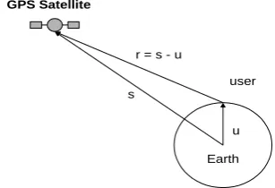
The signals transmitted by the GPS satellites are used to measure the Time of Arrival (TOA) at the receiver. Since the propagation speed (the speed of light) is known, the distance (geometric range) can be calculated from the delay.
GPS Satellite
user r = s - u
s
u
Earth
Figure 1. Definition of the User-to-Satellite vector r
is located at position , the user-to-satellite vector can then be written as shown in Fig. 1.
(2)
III. GPSERROR SOURCES
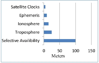
As depicted in eq. 1, there are a number of possible sources of errors which can degrade the accuracy of position computed and hence adversely affect the performance of a GPS receiver. These error sources can be mainly categorized into two groups, system wide errors and specific operating environment or specific GPS receiver errors. System wide errors include selective availability (S/A), ephemeris error, satellite clock error, troposphere and ionosphere error. We shall only discuss the troposphere error effect in the paper. System wide errors and their impact which can be reduced partially or completely eliminated by means of differential correction technique are summarized in the following Fig. 2.
Figure 2. System wide errors and their impact
IV. TROPOSPHERIC ERROR
Troposphere is the initial part of atmosphere and ranges up to 16 km in altitude from the surface of the earth, although the neutral atmosphere extends up to 60 km [5]. The Troposphere affects the GPS signals which are in fact electromagnetic waves, to a significant level. As a result the GPS signals are both delayed and refracted. The main factors which cause troposphere delay include temperature, pressure and humidity. The delay also varies with the height of the user position as the type of terrain below the signal path can affect the delay. According to Hopfield [6], there are two components of troposphere delay, namely wet delay and dry delay. The dry component which comprises of about 80 to 90% of the total delay is easier to determine as compared to the wet component.
TABLE I. TROPOSPHERIC DELAY ON MEASURED RANGE
S.No Elevation angle in degree Dry component (in meters) Wet Component (in meters) Total Delay (in meters)
A. 900 2.3 0.2 2.5
B. 200 6.7 0.6 7.3
C. 150 8.8 0.8 9.6
D. 100 12.9 1.1 14.0
E. 50 23.6 2.2 25.8
Table I depicts the average numerical values of both components of the troposphere delay related to different elevation angles.
The dry delay is mainly caused by the O2 and N2 gases
present in the atmosphere and it can be modeled only up to1% or better. On the other hand the wet delay which causes up to 10-20% of the total delay is difficult to model. The wet delay is due to the presence of water vapors in the atmosphere. Mathematically the tropospheric delay T can be represented as
∫ ( ) (3)
where is the refractive index of the atmospheric gases and is the difference between the curved and free-space paths.
During the last several decades, number of models (Hopfield model, Saastamoinen model, etc) have been developed and reported in scientific literature by researchers for estimation and correction of the delay induced by the troposphere in the GPS signal. However, much research has gone into the creation and testing of tropospheric refraction models to compute the refractivity N along the path of signal travel. Among these models the Hopfield model is most commonly used.
A. Hopfield Model
Hopfield [7] developed a dual quadratic zenith model of the refractivity with different and separate quadratics for the dry and wet atmospheric profiles. He described that refractivity is function of height above the surface assuming single polytrophic layer. The following formula is adopted by the model:
( ) (4)
( )
where is the total zenith atmospheric delay the top height of the dry atmospheric layer, height of the wet atmospheric layer, ground atmospheric pressure (mbar), ground temperature (T ), ground water vapor pressure and height of the ground level of the observing station, the constant parameters are k1 =77.6 K/mbar, k2 = 71.6 K2/mbar and k3 = 3.747 ×10⁵ K2/mbar.
V. SIMULATION AND RESULTS
The simulation work was carried out in the software Matlab version 7.3 on actual acquired GPS data. The sequence of steps carried out during the simulation process is explained in the following subsection.
A. Capturing of GPS Data
window during measurements to have a good view of the sky. The GPS signals were received, amplified, down-converted, and digitized into base band samples. The base band samples are then processed using software routines to acquire and track the direct GPS signal and to generate the receiver position information as explained in following sections. The software receiver can perform signal acquisition and tracking, navigation data extraction, code offset calculations and more importantly the parameters can be conveniently changed and the receiver can be adapted to suit different conditions [9].The available satellites were limited to five on the particular afternoon, when measurements were performed. They were however enough to perform the tracking and position calculations as mentioned below in the subsection c.
B. Analysis of GPS Data
The analysis of the data started with the generation of two types of plots as shown in the Fig. 3. The first plot in the figure depicts the time domain plot for 1000 samples of data. The GPS signal is transmitted using DSSS techniques, hence, as expected no discernible structure is visible, despite the 4.78 MHz IF present in the frequency domain plot.
Figure 3.Time and frequency domain plots for the actual GPS data
C. Acquisition and Tracking of Satellites
The first step in the simulation was to acquire the GPS satellites from the captured data. The acquisition plot for the captured GPS data is shown in Fig. 4. Only four satellites have strength greater than the acquisition threshold set at 2.5. This is an arbitrary level and can be revised based on the circumstances. The purpose of the acquisition process is to identify if a certain satellite is visible or not. If the satellite is visible, the acquisition process determines the coarse values of carrier frequency and code phase of the satellite signals.
The parameters i.e. carrier frequency and code phase are further refined by the tracking process. The main purpose of tracking algorithms is to refine the coarse values of code phase and frequency, and keep track of these as the signal properties change over time. Thus the tracking code runs continuously to follow the changes in
frequency as a function of time in order to keep the signal locked and decode the navigation data.
Figure 4. Acquisition results
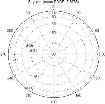
C. Satellites Tracked
The sky plot in Fig. 5 shows which satellites were visible and tracked when GPS data was captured. The satellites are shown using their PRN number inside the figure.
Figure 5. Satellite sky plot
D. Function Tropo
This Matlab subroutine is based on Hopfield tropospheric model [6]. The tropospheric correction model used in the simulation was selected because it gives best results as compared to other tropospheric models and is used widely for tropospheric correction. The model calculates tropospheric correction which is used for correction of computed user position. Correction in meters is stored in variable ddr. The range correction ddr in m is to be subtracted from pseudo-ranges and carrier phases. Descriptions of some important parameters of the Tropospheric correction function giving in Table II.
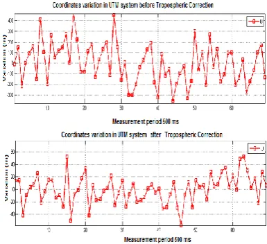
E. Position before and after Tropospheric Correction
to Fig. 8. Difference in latitude value was noted and also a significant variation can be seen in coordinates in UTM system from these figures. Results for 70 ms (millisecond) out of 500 ms (millisecond) data are shown in the Fig. 6 to Fig. 8.
Figure 6. East coordinate variations with and without tropospheric correction
Figure 7. North coordinate variations with and without tropospheric correction
Figure 8. Uping coordinate variations with and without tropospheric correction
TABLE II.DESCRIPTION OF IMPORTANT PARAMETERS OF TROPO
FUNCTION
S/N Parameter Description
1. sinel sin of elevation angle of satellite.
2. hsta Height of station in km.
3. p Atmospheric pressure in mb at height hp.
4. tkel Surface temperature in degrees Kelvin at height htkel.
5. hum Humidity in % at height hhum. 6. hp Height of pressure measurement in km.
7. htkel Height of temperature measurement in km.
8. hhum Height of humidity measurement in km.
VI. CONCLUSION
This paper has demonstrated the impact of tropospheric effect on GPS positioning. As shown in the simulation and results section, the tropospheric error can degrade the GPS receiver accuracy up to significant level if the error is not compensated properly. Further research can be carried out by capturing more GPS data and analyzing the results.
ACKNOWLEDGMENT
The authors would like to thank Higher Education Commission (HEC), Pakistan for the financial support of thiswork.
REFERENCES
[1] E. D. Kaplan and C. J. Hegarty, Understanding GPS Principles and Application, 2nd ed. Artech House Publishers London, 2005, ch 1.
[2] G. Lachapelle, A. Bruton, J. Henriksen, M. E. Cannon, and C. McMillan, “Evaluation of high performance multipath reduction technologies for precise DGPS shipborne positioning,” The Hydrographic Journal, no. 82, pp. 11-17, October 1996.
[3] L. Baroni and H. K. Kuga, “Analysis of navigational algorithms for a real time differential GPS system,” in Proc. 18th International Congress of Mechanical Engineering, Ouro Preto, MG, November 6-11, 2005.
[4] D. Wells, et al. Guide to GPS Positioning, 2nd ed. Canadian GPS
Associates, 1987.
[5] C. Satirapod and P. Chalermwattanachai, “Impact of different tropospheric models on GPS baseline accuracy: Case study in Thailand,” Journal of Global Positioning Systems, vol. 4, no. 1-2, pp. 36-40, 2005.
[6] H. S. Hopfield, “Tropospheric effects on electromagnetically measured range: Prediction from surface weather data,” Radio Science, vol. 6, no. 3, 1971.
[7] H. S. Hopfield, “Two–quadratic tropospheric refractivity profile for correction satellite data,” Journal of Geophysical Research, vol. 74, no. 18, pp. 4487 – 4499, 1969.
[8] M. Usman and D. W. Armitage, “Acquisition of reflected GPS signals for remote sensing applications,” in Proc. ICAST, Islamabad, Pakistan, 29-30 November, 2008,
Tahir Saleem was born in KPK, Pakistan. He received the BS degree in Information Technology from Kohat University in 2006 and the M.S.E degree in Electronic Engineering from International Islamic university Islamabad (IIUI) in 2010.Currently he is Ph.D scholar at IIUI in Electronic Engineering. His research interests focus on satellite communication and synthetic Aperture Radar (SAR) signal processing.
Mohammad Usman was born in Punjab, Pakistan.