Optimizing naturally driven air flow in a vertical pipe by changing the
intensity and location of the wall heat flux
M. Rahimia,* and M. Khalafi-Salouta a
Faculty of Engineering, University of Mohaghegh Ardabili, Ardabil, Iran
Article info: Abstract
Heat transfer from the internal surfaces of a vertical pipe to the adjacent air gives rise to the air flow establishment within the pipe. With the aim of optimizing the convective air flow rate in a vertical pipe, the details of the flow and thermal fields were investigated in the present study. Conservation equations of mass, momentum, and energy were solved numerically using simple implicit forward-marching finite difference scheme for a two-dimensional axis-symmetric flow. In order to evaluate and optimize the air flow rate passing through the pipe, the position and intensity of the wall heat flux were altered when the total employed heat transfer rate was constant. Based on the results of the numerical analysis, relatively more air flow rate was achieved when more intensified heat flux was employed at the lowest part of the vertical pipe. This finding was then validated using a simple experimental setup. The results of the present study could be useful in the design and application of buoyancy-assisted natural ventilation systems. Received: 25/01/2015
Accepted: 30/11/2015
Online: 03/03/2016
Keywords:
Natural ventilation, vertical pipe, wall heat flux.
Nomenclature
D Diameter of the vertical pipe (m)
g Gravity acceleration (9.81 m/s2)
l Mixing length (m)
L Length of the vertical pipe (m)
P Pressure (pa)
Pr Prandtl number
r Radial coordinate
R Pipe internal radius (m)
RR Gas constant for air (287 J/kg-K)
T Temperature (K or °C)
u Axial velocity component (m/s)
v Radial velocity component (m/s)
z Axial coordinate
Greek symbols
ρ Density (kg/m3)
µ Dynamic viscosity (N.s/m2)
σt Turbulent Prandtl number
τ Shear stress
Subscripts
a Surroundings
c Center
i Inlet
t Turbulent
w Wall
1. Introduction
solar chimneys have been developed. Specifications of air flow and heat transfer in a solar chimney have been investigated in many theoretical and experimental studies. Lee and Yan [1] studied laminar natural convection established between two vertical parallel plates, in which a uniform wall heat flux or uniform temperature was supposed to be applied in the middle part of the plates and thermal insulation was used in the rest. Based on the results, a correlation was proposed for the Nusselt number distribution over the plates. In a similar study, Lee [2] investigated laminar natural convection heat and mass transfer in an open vertical rectangular duct with uniform wall temperature or uniform wall heat flux boundary conditions. Analytical solutions were derived for the induced flow rate. Nusselt and Sherwood numbers under fully developed condition and correlation equations were also proposed for the relevant parameters.
Awbi [3] discussed the required parameters for designing natural ventilation systems and presented a procedure for calculating the air flow rate due to the wind and buoyancy effects. Bansal et al. [4] developed a mathematical model for a solar chimney under steady conditions. Varying discharge coefficients accounting for the openings with various sizes were taken into consideration in this model. Bansal et al. [5] examined the concept of a solar chimney coupled with a wind tower to enhance natural ventilation. It was theoretically estimated that the effect of a solar chimney was relatively much higher than that of the wind tower for lower wind speeds. Ong [6] proposed another mathematical model of a solar chimney which was physically similar to that of a Trombe wall. In this model, one side of the chimney was provided with a glass cover. This cover along with the other three solid walls formed a channel, through which the heated air could rise and flow by natural convection. Openings provided at the bottom and top of the chimney allowed the room air to enter and leave the channel. Using a thermal resistance network, steady state heat transfer equations were set up to determine the boundary temperatures in the
absorbing wall, and the air flowing within the channel.
Natural convection heat transfer in a vertical flat-plate solar air heater was experimentally studied by Hatami and Bahadorinejad [7]. Using the results, a correlation was suggested for the Nusselt number as a function of the Rayleigh number. The maximum efficiency was also found for the case in which the air heater had two glass covers and air could flow in all the channels. Arce et al. [8] experimentally investigated the thermal performance of a solar chimney employed in the natural ventilation of buildings. They deduced that the air flow rate passing through a solar chimney was mainly influenced by the pressure difference between the input and output, caused by thermal gradients and wind velocity. The discharge coefficient of 0.52 was also proposed for solar chimneys, which could be useful in the mass flow rate evaluation. Rahimi and Bayat [9] investigated the specifications of buoyancy-induced heated air flow within a vertical pipe. Air from the surroundings was directed into a heating chamber connected to a vertical pipe to establish a flow within the pipe. Air flow rate was evaluated using the measured velocity and temperature profiles. A model was developed for predicting the induced air flow rate, in which the predictions of the model were consistent with the experimental data over the tested range of the parameters.
first evaluated numerically. The results were then examined using a laboratory model to ensure the prediction of the numerical analysis. The implication of the study could be useful in the design and application of buoyancy-assisted natural ventilation systems.
2. Physical model
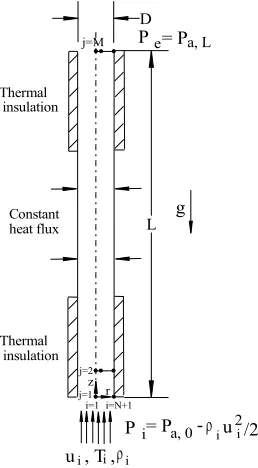
The physical model considered in the present study consisted of a vertical pipe with diameter D and length L, as shown in Fig. 1. In addition to the no slip velocity condition on the solid walls, thermal insulation boundary condition was applied for the surfaces of the pipe, except for a specified section, on which a uniform wall heat flux was employed. Uniform temperature and velocity profiles were assumed to exist at the inlet of the pipe and the inlet pressure was calculated using Bernoulli's equation. Hydrostatic pressure variation at constant temperature was supposed for the surroundings. Static pressure in the exit section of the pipe was also considered the same as that of the surrounding pressure at that altitude. The air was treated as an ideal gas with constant physical properties. The following conservation equations were used to describe the steady air flow developing within the pipe.
+1 ( )= 0 (1)
in which u and v are the axial and radial velocity components respectively.
+ = − −
+1 ( + )
(2)
where RR is the gas constant for air, g is the acceleration of the gravity, and µ and µt are dynamic and eddy viscosities, respectively.
+ =1 + (3)
in which Pr and σt are the Prandtl numbers in the laminar and turbulent flows, respectively. In order to facilitate the computational procedure, prandtl mixing length theory was employed to evaluate the turbulent viscosity. For a turbulent flow established within a circular pipe, Reynolds stress originating from the velocity fluctuations could be expressed by the following expressions (Frisch [10]):
́ = − = − (4)
where l is the turbulence mixing length.
Fig. 1. Physical model and the computational domain.
Based on the theoretical assumptions, a linear variation was supposed for the total shear stress as:
= − + ́ ́ = (5)
Using Eqs. (4) and (5), the following expression is obtained for the axial velocity variation in the radial direction:
L D
r z
i=1 j=1
i=N+1 j=M
Thermal insulation
Thermal insulation
Constant heat flux
u , T ,i i j=2
i
Pe= Pa, L
=
− + 4
2
(6)
Bradshaw [11] proposed the following equation for the mixing length which was used for the flow region within the pipe, except for the viscous sub-layer close to the wall:
= 0.14 1 −4
7 −
3
7 (7)
In order to have a generalized equation applicable for the whole flow region, Eq. (7) is usually multiplied by a damping function. Hanna et al. [12] proposed an expression for such a damping function as:
= 1 −
.
1 − .
(8)
Therefore, the following equation could be used to calculate the mixing length at any arbitrary point within the turbulent pipe flow:
= 0.14 1 −4
7 −
3
7 . (9)
Finally, turbulent viscosity was calculated using:
= (10)
3. Numerical analysis
Conservation equations of the mass, momentum, and energy described in the foregoing section were solved using a simple implicit forward-marching finite difference scheme [13]. Convective terms in the axial direction were estimated using backward difference approximation where the second order central difference approximation was applied for the terms in the radial direction. As indicated in Fig. 1, a 2-D domain was
considered to perform the numerical analysis, in which subscripts i and j were used to specify the grid points in the radial and axial directions, respectively. Using these indexes, the algebraic form of the momentum conservation equation, for instance, was obtained as follows:
,
, − ,
∆ + ,
, − ,
∆ + ∆
= − , − ,
∆ −
,
,
+1( + ),
, − ,
∆ + ∆
+ 2
∆ + ∆
( + ), /
, − ,
∆
− ( + ), /
, − ,
∆
(11)
The discretized form of Eq. (3) was first employed to obtain the temperature distribution over the grid points specified by j
=2 using predefined temperature and velocity values at the entrance. An additional equation was also developed and included in the set of algebraic momentum equations to preserve the mass flow conservation in each section of the pipe. Static pressure along with the axial velocity components was then evaluated using the combined set of equations at the grid points specified by j = 2. Finally, the continuity equation was employed to determine the radial velocity components at the same points. Having known the parameters at the grid points specified by j = 2, the forgoing steps were repeated sequentially to proceed in the axial direction.
The following steps were used to complete the numerical analysis:
- The length and diameter of the vertical pipe along with the thermal boundary condition were defined.
- Uniform air temperature, Ti, was considered
at the inlet and uniform axial velocity, ui,
- The numerical method was employed to calculate the temperature, pressure, and velocity components at the next axial position denoted by j = 2 with the inlet section parameters. The density was then specified at each point with the temperature values. The pressure was constant at all the grid points located in the second axial position.
- The last step was sequentially applied in a forward marching manner to reach the end of the pipe.
- The static pressure at the exit of the pipe was compared with the surrounding hydrostatic pressure and the inlet velocity was altered accordingly. The numerical analysis was then repeated for the newly assumed inlet uniform velocity. The calculation procedures were terminated when a unique pressure value was obtained for the exit section and the surroundings.
Thus, appropriate uniform velocity was determined for the prescribed physical and geometrical parameters including the length and diameter of the pipe, inlet and the surrounding temperatures, and the employed thermal boundary conditions.
4. Results and discussion
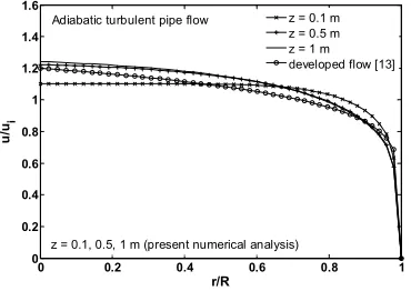
The numerical method described in the previous section was first applied to predict the developed pipe flow velocity profiles, for both laminar and turbulent regimes. A uniform velocity profile was assumed at the inlet of the pipe, based on which the inlet pressure was also specified. The developing flow was assumed to be incompressible and adiabatic at this stage. A number of the developing velocity profiles resulted from the present numerical analysis are presented in Figs. 2 and 3. The developed velocity profiles given by the following equations [14] for the two flow regimes were also sketched in these figures.
= 1 − = 2 1 − (12)
= 1 − =6
5 1 − (13)
Fig. 2. Velocity profiles for the laminar pipe flow.
It can be observed in Fig. 2 that the developed laminar velocity profile can be accurately predicted by the numerical analysis, but there was small diversity between the turbulent velocity profiles, as observed in Fig. 3. This discrepancy which was less than 10% was mainly due to the simple turbulence model used in the present analysis. Also, it is noteworthy that relatively shorter length was required for the turbulent pipe flow to be developed.
Fig. 3. Velocity profiles for the turbulent flow.
The values of the wall shear stresses both in the developed laminar and turbulent flow regimes were then used to perform systematic grid independency analysis. For this purpose, numerical analysis was applied for the prescribed pipe length and uniform inlet velocity, while the distance of the first grid point from the wall was varying at different analyses. The results of this analysis revealed that typical values of 1.1 mm and 0.2 mm
0 0.2 0.4 0.6 0.8 1
0 0.5 1 1.5 2 2.5
r/R
u
/ui
z = 0.1 m z = 1 m z = 2 m z = 4 m z = 6 m developed flow [13]
Z = 0.1, 1, 2, 4, 6 (present numerical analysis) Adiabatic laminar pipe flow
0 0.2 0.4 0.6 0.8 1
0 0.2 0.4 0.6 0.8 1 1.2 1.4 1.6
r/R
u
/ui
z = 0.1 m z = 0.5 m z = 1 m developed flow [13] Adiabatic turbulent pipe flow
could be reasonable for the minimum grid points separation in the laminar and turbulent flow analyses, respectively.
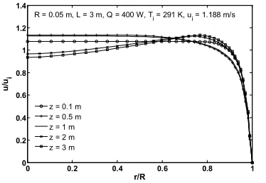
The numerical analysis was then employed for a vertical pipe with 3 m length and 0.1 m diameter. Also, the typical uniform wall heat flux of 400/(πDL) W/m2 was applied over the full length of the pipe. For the surrounding temperature of 291 K, the uniform inlet velocity of 1.24 m/s was obtained by completing the numerical procedure. For this illustrative configuration, the results of the numerical analysis as the velocity, temperature, and pressure distributions are shown in Figs. 4-6.
Fig. 4. Velocity profiles for the turbulent flow in a vertical pipe with uniform heat flux.
It is observed in Fig. 4 that the velocity profiles had a slight rise in the region close to the wall originating from the heat transfer process in that region. Unlike the velocity profile, Fig. 5 indicates that the flow temperature changed considerably both in the radial and axial directions. Also, constant and sharp temperature gradient existed in all the temperature profiles adjacent to the wall, which could represent the uniform wall heat flux. According to Fig. 6, static pressure in any section within the pipe was always less than the surrounding hydrostatic pressure. The pressure difference increased first in the flow direction due to the shear effect which was predominant compared with the buoyancy effect in the entrance region. The trend was gradually reversed getting far from the inlet
section and the pressure difference finally came up to zero in the exit section of the pipe.
Fig. 5. Temperature profiles for a turbulent flow in a vertical pipe with uniform heat flux.
Fig. 6. Pressure difference between the flow between the pipe and surroundings.
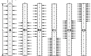
In order to optimize the air flow rate passing through the pipe, the intensity and position of the wall heat flux were altered, while the geometry of the pipe was constant. Various cases of the combined thermal boundary conditions are presented in Fig. 7, in which a symbol is allocated to each individual case. The case denoted by A represents the situation in which a uniform heat flux is applied over the entire surface of the pipe. Two cases denoted by B and C are the circumstances in which the total heat transfer rate is localized and applied to 2 m and 1 m length of the pipe, respectively. Also, the numerical suffixes refer to the different possible segments of the pipe, on which the localized heat flux is employed. Thermal insulation boundary condition is applied to the remaining surfaces of the pipe in all the cases.
0 0.2 0.4 0.6 0.8 1
0 0.2 0.4 0.6 0.8 1 1.2 1.4
r/R
u
/ui
z = 0.1 m z = 0.5 m z = 1 m z = 2 m z = 3 m
R = 0.05 m, L = 3 m, Q = 400 W, Ti = 291 K, ui = 1.188 m/s
0 0.2 0.4 0.6 0.8 1
0.9 1 1.1 1.2 1.3 1.4 1.5
r/R
T
/Ti
z = 0.1 m z = 0.5 m z = 1 m z = 2 m z = 3 m
R = 0.05 m, L = 3 m, Q = 400 W, Ti = 291 K, ui = 1.188 m/s
-1 -0.8 -0.6 -0.4 -0.2 0
0 0.5 1 1.5 2 2.5 3 3.5
p-psur (pa)
z
(
m
)
A B1 B2 C1 C2 C3 L
D
Fig. 7. Vertical pipe with different uniform and insulated thermal boundary conditions.
The numerical analysis was conducted to evaluate the air flow rate passing through the pipe under various circumstances. Figure 8 presents the resulted mass flow rates for different amounts of heat transfer rate and for various cases. For a constant heat transfer rate, it is seen in Fig. 8 that different amounts of air displacement through the pipe were obtained depending on the thermal boundary conditions. The localized heat flux applied in the lowest segment of the pipe gave rise to the maximum air mass flow rate passing throughout the pipe. In contrast, the minimum air displacement was achieved for this localized heat flux when applied in the uppermost segment of the pipe. Also, very close air displacement amounts were obtained for the two cases denoted by C2 and A.
Fig. 8. Air mass flow rate passing throughout the pipe for various heat transfer rates.
5. Experimental setup and findings
In order to examine the numerical predictions, an experimental setup including a vertical steel
pipe with 3 m length and 0.1 m diameter was assembled. A silicon heating wire was twisted round the pipe to heat up the pipe wall. The electrical resistance and length of the heating wire were 15 ohm/m and 12 m, respectively, and the total heat transfer rate of 270 W could be provided by this heating wire connecting it to the power supply unit. With the purpose of reducing the heat loss from the pipe to the surroundings, the external surface of the pipe was covered using a thermal insulating fabric with about 2 cm thickness. Various cases of the thermal boundary conditions presented in Fig. 7 were created by changing the density and location of the heating wire.
In order to evaluate the air flow rate passing through the pipe, the axial velocity component was measured at the entrance of the pipe using an accurate hot wire probe (DANTEC straight miniature model 55P11, 0-20 ±0.04 m/s). The probe was traveled with the very low speed of 1 cm/s along the pipe diameter and very close to the inlet section, and the data presenting the axial velocity component were being collected. With the purpose of having a sense from the temperature distribution in the developed flow, 8 k-type calibrated thermocouples were installed on a wire fixed along the diameter of the pipe and very close to the exit section. The thermocouples were closely spaced near the wall to measure sharp temperature gradient existing in that region. These thermocouples were connected to a data logging system to monitor and record the temperatures. A picture of the insulated pipe is presented in Fig. 9.
Fig. 9. A picture of the vertical insulated pipe.
200 300 400 500 600 700 800 900 1000
0.004 0.006 0.008 0.01 0.012 0.014 0.016
Q (W)
m
(
k
g
/s
)
A B1 B2 C1 C2 C3
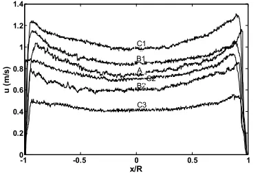
To start the experiment, the heating wire was connected to the power supply unit and a free convective flow was established within the pipe. The steady state of the flow was being checked by the exit temperature variations. The inlet axial velocity and the exit temperature variations were recorded under steady flow condition. The experiment was then repeated for different cases of the thermal boundary conditions examined in the numerical analysis. Figure 10 presents the velocity profiles obtained for different cases, in which the position and intensity of the wall heat flux were different. This figure indicates that a symmetrical air flow is established within the pipe in each case and, consistent with the numerical results, the air flow rate changes greatly depending on the thermal boundary condition of the pipe. Also, unlike the inlet uniform velocity assumption applied in the numerical analysis, Fig. 10 indicates that the velocity profiles are not quite uniform in this section, but have a small drop in the central region.
The thermocouple readings are presented in Fig. 11 under steady conditions and for various cases. According to this figure, more uniform temperature distribution existed in the exit section when applying the localized heat flux in the lower part of the pipe. In contrast, relatively higher temperature with sharp gradient close to the wall was measured for the case denoted by C3.
In order to compare the experimental and numerical results, the air flow rates were calculated using the recorded velocity profiles for the various cases. The corresponding air flow rates were also evaluated using the numerical analysis for the conditions of (L = 3 m, D = 0.1 m, Q = 270 W, Ta = 19°C and Pa =
86 kpa). The results were tabulated in Table 1. The data indicated that the experimental flow rates were somewhat lower than the numerical results for all the examined cases. A small part of this discrepancy was related to the assumptions made in the numerical analysis and the shortcomings existing in the experimental setup. However, this difference was mainly concerned with the heat loss from
recorded temperature data were insufficient to precisely evaluate this heat loss. In addition, the general trend in the variation of the air flow rate with the applied thermal boundary condition was strongly confirmed. Also, based on the specifications of the velocity and temperature measurement devices, ± 0.04 m/s and ±0.2°C uncertainties were expected in the provided data.
Fig. 10. Experimental velocity profiles at the inlet of the pipe (L = 3 m, D = 10 cm, Q1 = 270 W).
Fig. 11. Experimental temperature profiles at the exit of the pipe.
Table 1. Comparison of the air flow rate (kg/s)
Various
cases Experiments
Numerical analysis
Differences (%)
A 0.00584 0.00750 22.1
B1 0.00656 0.00841 22.0
B2 0.00464 0.00621 25.3
C1 0.00756 0.00927 18.4
C2 0.00540 0.00728 25.8
C3 0.00316 0.00444 28.8
-1 -0.5 0 0.5 1
0 0.2 0.4 0.6 0.8 1 1.2 1.4
x/R
u
(
m
/s
)
B2 B1 A C1
C2
C3
-1 -0.5 0 0.5 1
300 310 320 330 340 350 360
x/R
T
(
K
)
6. Conclusions
A vertical pipe or channel could be employed as a secondary ventilating system to discharge air from a space to the surroundings by warming up the air within the channel. It was found that the free convective air flow rate through a vertical pipe was quantitatively affected by the intensity and location of the wall heat flux. For a constant heat transfer rate provided by any arbitrary heat source, the more localized the heat flux utilized in the lowest part of the pipe, the more the air displacement would be achieved. In contrast, the localized heat flux led to a relatively small amount of air displacement when applied in the uppermost part of the pipe. Also, air displacement achieved by a uniform heat flux applied over the entire surfaces of the pipe was quite comparable with that of the localized heat flux applied in the middle part of the pipe.
References
[1] K. T. Lee, and W. M. Yan, “Laminar natural convection between partially heated vertical parallel plates”,Wärme- und Stoffübertragungb, Vol. 29, No. 3, pp. 145-151, (1994).
[2] K. T. Lee, “Laminar natural convection heat and mass transfer in vertical rectangular ducts”,Int. J. heat and mass transfer, Vol. 42, No. 24, pp. 4523-4534, (1999).
[3] H. B. Awbi, “Design considerations for naturally ventilated buildings”,
Renewable Energy, Vol. 5, No. 5-8, pp. 1081–1090, (1994).
[4] N. K. Bansal, R. Mathur, and M. S. Bhanduri, “Solar chimney for enhanced stack ventilation”, Building and Environment, Vol. 28, No. 3, pp. 373-377, (1993).
[5] N. K. Bansal, R. Mathur, and M. S.
Bhandari, “A study of solar chimney assisted wind tower system for natural ventilation in buildings”, Building and Environment, Vol. 29, No. 4, pp. 495-500, (1994).
[6] K. S. Ong, “A mathematical model of solar chimney”, Renewable Energy, Vol. 28, No. 7, pp. 1047-1060, (2003). [7] N. Hatami, and M. Bahadorinejad,
“Experimental determination of natural convection heat transfer coefficient in a vertical flat-plate solar air heater”, Solar Energy, Vol. 82, No. 10, pp. 903-910, (2008).
[8] J. Arce, M. J. Jimenez, J. D. Guzman, M. R. Heras, G. Alvarez, and J. Xaman, “Experimental study for natural ventilation on a solar chimney”,
Renewable Energy, Vol. 34, No. 12, pp.
2928-2934, (2009).
[9] M. Rahimi, and M. M. Bayat, “An experimental study of naturally driven heated air flow in a vertical pipe”,
Energy and Building, Vol. 43, No. 1, pp. 126-129, (2011).
[10] U. Frisch, Turbulence, Cambridge University Press, London, (1995). [11] P. Bradshaw, Turbulence,
Springer-Verlag, Berlin, (1978).
[12] O. T. Hanna, O. C. Sandal, and P. R. Mazet, “Heat and mass transfer in turbulent flow under condition of drag reduction”, American institute of
Chemical Engineering Journal, Vol. 27,
pp. 693-697, (1981).
[13] B. Carnahan, H. A. Luther and J. D. Wilkes, Applied Numerical methods, Wiley, pp. 298-301, (1969).
[14] Y. A. Cengel and J. M. Cimbala, Fluid
Mechanics, Fundamentals and