http://www.sciencepublishinggroup.com/j/ajtas doi: 10.11648/j.ajtas.s.2017060501.18
ISSN: 2326-8999 (Print); ISSN: 2326-9006 (Online)
Evaluation of Techniques for Univariate Normality Test
Using Monte Carlo Simulation
Ukponmwan H. Nosakhare, Ajibade F. Bright
Department of General Studies, Mathematics and Computer Science Unit, Petroleum Training Institute, Warri, Nigeria
Email address:
[email protected] (U. H. Nosakhare), [email protected] (A. F. Bright)
To cite this article:
Ukponmwan H. Nosakhare, Ajibade F. Bright. Evaluation of Techniques for Univariate Normality Test Using Monte Carlo Simulation. American Journal of Theoretical and Applied Statistics. Special Issue: Statistical Distributions and Modeling in Applied Mathematics. Vol. 6, No. 5-1, 2017, pp. 51-61. doi: 10.11648/j.ajtas.s.2017060501.18
Received: February 24, 2017; Accepted: March 1, 2017; Published: June 9, 2017
Abstract:
This paper examines the sensitivity of nine normality test statistics; W/S, Jaque-Bera, Adjusted Jaque-Bera, D’Agostino, Shapiro-Wilk, Shapiro-Francia, Ryan-Joiner, Lilliefors’and Anderson Darlings test statistics, with a view to determining the effectiveness of the techniques to accurately determine whether a set of data is from normal distribution or not. Simulated data of sizes 5, 10, …, 100 is used for the study and each test is repeated 100 times for increased reliability. Data from normal distributions (N (2, 1) and N (0, 1)) and non-normal distributions (asymmetric and symmetric distributions: Weibull, Chi-Square, Cauchy and t-distributions) are simulated and tested for normality using the nine normality test statistics. To ensure uniformity of results, one statistical software is used in all the data computations to eliminate variations due to statistical software. The error rate of each of the test statistic is computed; the error rate for the normal distribution is the type I error and that for non-normal distribution is type II error. Power of test is computed for the non-normal distributions and use to determine the strength of the methods. The ranking of the nine normality test statistics in order of superiority for small sample sizes is; Adjusted Jarque-Bera, Lilliefor’s, D’Agostino, Ryan-Joiner, Shapiro-Francia, Shapiro-Wilk, W/S, Jarque-Bera and Anderson-Darling test statistics while for large sample sizes, we have; D’Agostino, Ryan-Joiner, Shapiro-Francia, Jarque-Bera, Anderson-Darling, Lilliefor’s, Adjusted Jarque-Bera, Shapiro-Wilk and W/S test statistics. Hence, only D’Agostino test statistic is classified as Uniformly Most Powerful since it is effective for both small and large sample sizes. Other methods are Locally Most Powerful. Shapiro-Francia, an improvement of Shapiro-Wilk is more sensitive for both small and large samples, hence should replace Shapiro-Wilk while the Adjsted Jarque-Bera and the Jarque-Bera should both be retained for small and large samples respectively.Keywords:
Error Rate, Power-of-Test, Normality, Sensitivity, and Simulation1. Introduction
Normality tests are used to determine whether a set of data could be modeled by a normal distribution or to investigate whether a set of observations is normally distributed. Statistical methods can be classified into two; parametric and nonparametric methods. Parametric methods such as Student-t Student-tesStudent-t and Analysis of Variance require Student-thaStudent-t Student-the seStudent-t of daStudent-ta Student-to be used is normally distributed, otherwise, the tests become invalid. Nonparametric tests such as Friedman test, Kruskal-Wallis test, Mann-whitney test, etc require no assumption on the distribution of the data. According to Nornadiah and Yap (2011), normal distribution is the underlying assumption of many statistical procedures, hence, the need for normality
test in the field of statistical inference. In testing for normality, the primary aim is to investigate whether or not available (sample) data was drawn from a normally distributed population. In some cases, where real life data do not satisfy the necessary parametric assumptions, researchers transform such data to adjust for normality and other basic assumptions of parametric tools such as homogeneity of variance (Seth, 2008; Jason, 2002; Jason, 2010; Pitchaya et al, 2012).
quantile-quantile plot (Q-Q plot), histogram, box-plot and stem-and-leaf plot. Analytical test for normality testing involves the use of mathematical formulae, this include Shapiro-Wilk test, Jarque-Bera test, Kolmogorov-Smirnov test, Ryan-Joiner test etc. Many researchers, especially those with phobia for mathematics, apply or prefer graphical approach because it requires less formula and can easily be understood, even by the beginner in research.
Statistical tests generally have limits where they tend to be weak and unsuitable for what they are meant for. Normality tests are numerous with significant variations in terms of sensitivity as the powers of the tests vary significantly and even produce unequal p-value using the same set of data. This implies the inability of some of the normality tests to detect the actual distribution of a set of data which could lead to either type I or type II errors.
Statistical tests that can stand the test of time and applicable in every situation with minimal error are referred to as Uniformly Most Powerful (UMP) and those that can only perform excellently in a defined environment or condition are referred to as Locally Most Powerful (LMP) (Piegorsch and Bailer, 2005). Due to the proliferation of normality tests, the sensitivity of tests could vary significantly based on some factors such as parameters of the available or sampled data like mean, skewness, kurtosis, sample size, etc. Based on the definition given by Piegorsch and Bailer (2005), normality tests that are consistent irrespective of sample size are here referred to as UMP while those that are adopted for some specified sample sizes, either small or large, are referred to as LMP.
Recently, many researchers investigated the strength of some normality techniques and their adequacy in the detection of normality of sets of data. Ryan (1990) faults his previous research by concluding that the method proposed in his earlier research can only be used perfectly for small sample sizes. Also, Shapiro and Francia (1976), proposed another method called Shapiro-Francia due to the incompetence of the first proposed method of test of normality by Shapiro and Wilk (1965) called Shapiro-Wilk. In like manner, Jarque-Bera test was proposed by another researcher who strictly considered kurtosis and skewness as measures of normality of a set of data and later modified the method to form Adjusted Jarque-Bera test.
Inaddition, many researchers have investigated the competencies of some of the existing methods due to the proliferation of normality tests and there exists significant variations in their conclusions as seen in the results of Yap and Sim (2011), Nornadiah and Yap (2011), Panagiotis (2010) and Mayette (2013). Researchers such as Stephen (1974), Douglas and Edith (2002), Siddik (2006), Derya et al (2006), Frain (2006), Nor-Aishah and Shamsul (2007), Rinnakorn and Kamon (2007), Zvi et al (2008), Nornadiah and Yap (2011), Yap and Sim (2011), and Shigekazu et al (2012) have investigated the sensitivity of various normality techniques using power of test by simulating data from desirable distribution. Most of the works failed to categorize the methods based on sample size and in terms of peakedness and skewness of the data.
Hence, this paper which aims at evaluating the performance of some existing normality techniques with regards to a wide range of sample sizes and distributions, with a view to classifying them into Uniformly Most Powerful (UMP) and Locally Most Powerful (LMP) tests.
2. Review of Normality Techniques
Investigated
2.1. Shapiro-Wilk Statistic (W) Normality Test
According to Farrel and Stewart (2006), Shapiro-Wilk statistic is based on order statistics of the sample, the case weights have to be restricted to integers. The W statistic is defined as:
(
)
(
)
2
(1)
2
( ) 1
1 n
i i
x x
n W
n
x x
− − =
−
−
∑
(1)
where x(1)≤x( 2) ≤ ≤... x( )n are ordered sample values, n is
the sample size and 1
n i i
x x
n
=
=
∑
is the mean. Critical value ofW is available in a statistical table and decision is based on the comparison of the W statistic value and the critical value. The null hypothesis is rejected if the critical value is less than the statistic W.
2.2. Shapiro-Francia Test
According to Royston (1983), the Shapiro-Francia Test statistic (W′) is computed using
( )
2
( ) 1
2 2
1 1
n i i i
n n
i i
i i
m x W
m x x
=
= =
′ =
× −
∑
∑
∑
(2)
Where xi is the ordered observed values arranged in ascending order and mi is the vector of the expected values of standard normal order statistics. x is the mean of the observed values.
Critical value of W′ is available in a statistical table and decision is based on the comparison of statistic and the critical value. The null hypothesis is rejected if the critical value is less than the statistic W′.
2.3. Jarque-Bera Normality Test
The Jarque-Bera test is a goodness-of-fit test of whether sample data have the skewness and kurtosis matching a normal distribution. The test is named after Carlos Jarque and Anil K. Bera (1980). The test statistic JB is defined as
(
)
22 1
3
6 4
n
JB= S + k−
where n is the number of observations (sample size); S is the sample skewness, and k is the sample kurtosis:
( ) ( ) 3 3 1 3 3 2 2 1 1 1 n i i n i i x x n S x x n µ σ = = − = = −
∑
∑
(4)and
(
)
(
)
4 1 4 4 2 2 1 1 1 n i i n i i x x n K x x n µ σ = = − = = − ∑
∑
(5)where µ3 and µ4 are the estimates of third and fourth central
moments respectively, x is the sample mean, and
σ
2is the estimate of the second central moment, the variance. The calculated value is compared with the table value using Chi-Square distribution table at a desirable level of significance (usually 0.05). The decision rule is; accept the null hypothesis if the table value is greater than the calculated value, otherwise, reject.
2.4. Modified/Adjusted Jarque-Bera (AJB) Test Statistic
In the modified Jarque-Bera test statistic, the computation of both skewness and kurtosis differ from the previous Jarque-Bera test statistic as modified by Urzua (1996). Here, the Skewness (g1) is;
(
)(
)
(
)
( )
3 2 3 1 1 2 1 2 n i i x x n gn n s
= − = − −
∑
(6)where n is the sample size, s is the standard deviation, xi is
the ith observation and x is the mean (average observation) of the observed data. The kurtosis (g2) is computed using;
(
)(
)
4 2
2
1
( 1) 3( 1)
1 2 ( 3) ( 2)( 3)
n i i
x x
n n n
g
n n n = s n n
−
+ −
= − − − − − −
∑
(7)Then, AJB becomes;
( )
2( )
2( ) ( )
1 2 2 21 2
1
6 4 6 24
g g
n
AJB g g n
= + = +
(8)
The decision rule is; accept the null hypothesis if the table value is greater than the calculated value, otherwise, reject H0.
2.5. Ryan-Joiner Normality Test
According to Ryan (1976), the test assesses normality by calculating the correlation between sample data and its normal scores. If the correlation coefficient is close to 1, the population is said to be normal. The Ryan-Joiner statistic assesses the strength of this correlation; if it falls below the appropriate critical value, reject the null hypothesis of
population normality.
Considering set of observations; x where ii =1, 2, ...,n , the z-score of the set of observations is i x
i x x m z s − =
where mx is the mean of the set of observations and sxis the
standard deviation of the observations. By definition,
( )
cov , ( ) x y x y Correlation r σ σ= (9)
To test:
H0: r is insignificant (r = 0) versus
H1: r is significant (r
≠
0) Using the test statistic:2 2 1 calculated n t r r − =
− (10)
2
1 , 2
tabulated n
t =t−α − (11)
the null hypothesis is rejected if the tcalculated > ttabulated value, otherwise, it is accepted. Using p-value, the null hypothesis is rejected if the p-value is less than the level of significance of the test (0.05). Then, for the test of normality, the hypothesis is accepted if the “r” is significant.
2.6. D’Agostino D Test
According to D’Agostino and Stephen (1986), the test statistic can be used to detect departure of data set from normality. It requires that the observations be ordered in ascending order and the mean deviations of the ordered data, used to compute Dcalculated which was compared with the range/interval of values from table values of D (Dtabulated). The null hypothesis is rejected if the Dcalculated value falls outside the range of values from the D’Agostino critical values, otherwise, it is accepted. The test statistic is;
3 T D
n SS
= (12)
Where 1 1 2 n i i n
T i x
=
+
= −
∑
(13)(
)
2 1n i i
SS x x
=
=
∑
− , xi is the ith observation and n = sample2.7. W/S Test
The test uses sample standard deviation and the data range which is the difference between maximum observation and the minimum observation. The test statistic is expressed as;
w q
s
= (14)
where w is the range of available set of data and ‘s’ is the sample standard deviation.
1 2 2
1
( )
1
n i i
x x
s
n
=
−
=
−
∑
(15)
The critical value is read from W/S normality test table which has boundary values a and b, where a is the lower boundary or the left-sided critical values and b is the upper boundary or the right-sided critical value. The null hypothesis is rejected if the calculated q value falls outside the boundary of the table values, otherwise, it is accepted.
One of the advantages of the test is that it can be used for even samples size less than 5 as the table has the least value as low as 3.
2.8. Modified Kolmogorov-Smirnov Normality Test (Lilliefor’s Test)
Modified Kolmogorov-Smirnov test is a non-parametric test for equality of continuous probability distributions which can be used to compare a sample with reference probability distribution or to compare two samples (Wikipedia, 2013). Kolmogorov-Smirnov statistic quantifies the distance between the empirical distribution function of the sample and the cumulative distribution function of the reference distribution, or between the empirical distribution functions of two samples. If the observed difference is sufficiently large, the test will reject the null hypothesis of the population normality. The test statistic is given as;
[
]
1 0 1
( )i ( ) , ( )i i ( i ) ,
L=Maxℓ z −N z ℓ z −N z− =Max D D− (16)
Where i i x x
x m
z s
−
=
x
s is the standard deviation of the set of observations, mx
is the mean and xi is the ith observation. ℓ( )zi is the
proportion of scores smaller than Zi and N z( )i is the
cumulative probability associated with Zi for the standard normal distribution. Therefore, L is the maximum absolute value of the biggest difference between the probability associated to zi when zi is normally distributed and the
observed frequency (ℓ( )zi ). The null hypothesis of normality
is rejected when the L value is greater than or equal to the critical value (Molin and Abdi, 2007).
2.9. Anderson Darling Test
According to D'Agostino and Stephen (1986), the test compares the Empirical Cumulative Distribution (E.C.D) function of sample data with the distribution expected. If this observed difference is sufficiently large, the test will reject the null hypothesis of population normality. The test statistic is a squared distance that is weighted more heavily in the tails of the distribution. The Anderson-Darling normality test statistic is given as:
(
)
(
)
(
1)
2 1
ln ( )i ln 1 n i
i
AD n F x F x
n + −
−
= − − + −
(17)
*
2 0.75 2.25 1
AD AD
n n
= + +
(18)
Where F is the cumulative distribution function of the normal distribution and xi is the ordered observations.
3. Yardstick for Classification of
Normality Techniques into UMP and
LMP
The study involves both small and large sample sizes. Normality testing techniques that can detect normality of a set of data irrespective of the sample size, either small or large will be referred to as UMP but those that are better for either of small or large sample size will be categorized as LMP. This implies that any normality testing technique classified as UMP can be used by researchers for test of normality, irrespective of sample size of the data.
4. Source and Sample Size of the Data
Simulation was used in the generation of the required data using defined statistical distributions with known parameters. Symmetric distributions such as normal distribution; N(2,1) and N(0,1), Student-t distribution (8), Cauchy distribution (7, 3), and asymmetric distributions such as Chi-square distribution (χ2(4)
), and Weibull distribution [7,3] were used in the simulation of data. Since the sample space of the parameter values are unlimited, the values were chosen randomly since from the literature, the methods have similar behaviour irrespective of the parameters of the distributions considered. (Siddik, 2006; Normadiah and Yap, 2011; Yap and Sim, 2011; Marmolejo-Ramos and Gonza’Lez-Burgos, 2012).
Also from literature, it is confirmed that at sample size of 100 and above, the normality techniques have the same behaviour and sensitivity to both normally distributed and non-normally distributed data (Ryan and Joiner, 1976; Derya et al, 2006; Normadiah and Yap, 2011, Nor-Aisha et al., 2007 and Mayette and Emily, 2013; Abbas, 2013), therefore, maximum sample size considered in this study is 100.
5. Algorithm for Monte Carlo Simulation
simulation is used to determine the performance of an estimator or test statistic under various scenarios. The structure of a typical Monte Carlo exercise is as follows:
1.Specify the “Data Generation Process”. 2.Choose a sample size N for the MC simulation.
3.Choose the number of times to repeat the MC simulation.
4.Generate a random sample of size N based on the Data Generation Process.
5.Using random sample generated in 4 above, calculate the statistic(s).
6.Go back to (4) and repeat (4) and (5) until desirable replicate is achieved.
7.Examine parameter estimates, test statistics, etc.
6. Determination of Sensitivity of
Normality Techniques
The P-value was used in the study of sensitivity of normality testing techniques considered. In statistical analysis, the p-value defines the point at which the test starts being significant. The decision rule is to reject the null hypothesis if the p-value is less than the level of significance. In this study, a p-value greater than level of significance implies the set of data is normally distributed and the higher the value, the more sensitive the statistic used among the rest provided the data is simulated using normal distribution..
According to Nornadiah and Yap (2011), power of a statistical test is the probability that the test will reject the null hypothesis when the alternative hypothesis is true (i.e. the probability of not committing a Type II error). The power is in general a function of the possible distributions, often determined by a parameter, under the alternative hypothesis. As the power of test increases, the chance of a Type II error occurring decreases. The probability of a Type II error occurring is referred to as the false negative rate (β). Therefore power of test is equal to 1 − β, which is also known as the sensitivity (Gupta, 2011).
7. Data Analysis
This section deals with analysis of simulated data from symmetric and asymmetric distributions using nine selected normality test methods (univariate methods). The data analysis involves following steps;
1.Simulate data of sizes n =5, 10,..., 100 from the six distributions; N(2,1), N(0,1), Weibull (7,3), 2
(4) χ , t(8), and Cauchy (7,3).
2.For each sample size, n, replicated 100 times,
i Calculate the normality test statistics for each of the nine univariate normality tests
ii Reject/Accept the null hypothesis; H0: the data are normally distributed. H1: the data are not normally distributed.
iiiCalculate the error rate =
(100) number of times wrong decision is recorded
number of replicate
ivCalculate the type I error or power of test = 1−p type II error( )
See Tables 1 to 9 for the error rates obtained for the nine normality tests methods.
8. Error Rates
Table 1. Error Rate of W/S Test Statistic.
Asymmetry Symmetry
N[2,1)] N[0,1] Weibull 7(3)
Chi-Sqr.(4) t(8) Cauchy(7,3) 5 0.10 0.03 0.91 0.86 0.91 0.92 10 0.11 0.08 0.88 0.97 0.89 0.71 15 0.07 0.09 0.91 0.91 0.80 0.48 20 0.07 0.07 0.82 0.94 0.79 0.25 25 0.08 0.06 0.88 0.81 0.76 0.17 30 0.07 0.08 0.87 0.85 0.85 0.14 35 0.13 0.06 0.92 0.85 0.77 0.08 40 0.08 0.09 0.91 0.82 0.78 0.04 45 0.10 0.05 0.89 0.90 0.65 0.04 50 0.11 0.05 0.88 0.78 0.76 0.01 55 0.12 0.06 0.86 0.78 0.79 0.01 60 0.12 0.06 0.76 0.79 0.70 0.01 65 0.10 0.07 0.78 0.81 0.71 0.01 70 0.13 0.08 0.84 0.83 0.73 0.02 75 0.08 0.08 0.75 0.76 0.66 0.00 80 0.11 0.08 0.79 0.77 0.69 0.01 85 0.11 0.07 0.73 0.76 0.65 0.00 90 0.06 0.09 0.77 0.78 0.64 0.00 95 0.13 0.07 0.78 0.79 0.60 0.00 100 0.06 0.08 0.74 0.82 0.62 0.00
From Table 3, it can be seen vividly that the test is highly inconsistent as the error rate is considerably high irrespective of the sample sizes and for all the distributions except Cauchy (7, 3). However, the behaviour of the test is different for t-distribution which belongs to the same category as Cauchy distribution highlighting the inconsistency of W/S test.
Table 2. Error Rate of JB Test Statistic.
Asymmetry Symmetry
N[2,1] N[0,1] Weibull 7(3)
Chi-Sqr.(4) t(8) Cauchy(7,3)
5 0.00 0.00 1 1 1 1
Asymmetry Symmetry
N[2,1] N[0,1] Weibull 7(3)
Chi-Sqr.(4) t(8) Cauchy(7,3) 95 0.02 0.03 0.70 0.00 0.63 0.00 100 0.01 0.03 0.70 0.00 0.58 0.00
From Table 2 the error rate of Jarque-Bera test decreases as the sample size increases, an indication that the method is more active or efficient for large sample size especially for the non-normal distributions.
Table 3. Error Rate of AJB Test Statistic.
Asymmetry Symmetry
N[2,1] N[0,1] Weibull 7(3)
Chi-Sqr.(4) t(8) Cauchy(7,3) 5 0.03 0.05 0.03 0.04 0.07 0.71 10 0.02 0.03 0.05 0.17 0.05 0.41 15 0.04 0.05 0.07 0.24 0.11 0.18 20 0.04 0.05 0.06 0.35 0.13 0.16 25 0.05 0.02 0.06 0.37 0.18 0.10 30 0.05 0.05 0.04 0.53 0.14 0.09 35 0.08 0.08 0.12 0.61 0.23 0.01 40 0.04 0.03 0.14 0.73 0.82 0.00 45 0.08 0.05 0.23 0.75 0.70 0.01 50 0.01 0.02 0.20 0.73 0.71 0.00 55 0.09 0.05 0.22 0.89 0.68 0.00 60 0.10 0.05 0.17 0.90 0.68 0.01 65 0.05 0.04 0.28 0.89 0.69 0.01 70 0.03 0.05 0.20 0.93 0.67 0.01 75 0.03 0.04 0.20 0.88 0.63 0.00 80 0.05 0.04 0.18 0.94 0.65 0.00 85 0.02 0.02 0.16 0.96 0.65 0.00 90 0.02 0.01 0.26 0.97 0.60 0.00 95 0.02 0.03 0.31 1.00 0.62 0.00 100 0.03 0.03 0.31 1.00 0.55 0.00
For the non-normal distribution, error rate increases as sample size increases except for the Cauchy (7, 3). For the normal distribution, there is no impact of sample size on the error rate. It was observed that the error rate is significantly reduced for small sample sizes for the non-normal distributions for the ADJ test statistic, an indication that the adjusted Jarque-Bera Test is an improvement on the Jarque-Bera test for small sample sizes.
Table 4. Error Rate of D’Agostino Test Statistic.
Asymmetry Symmetry
N[2,1] N[0,1] Weibull 7(3)
Chi-Sqr.(4) t(8) Cauchy(7,3)
5 - - - -
10 0.05 0.04 0.53 0.64 0.73 0.15 15 0.04 0.04 0.53 0.59 0.72 0.18 20 0.06 0.05 0.52 0.71 0.74 0.15 25 0.04 0.05 0.52 0.68 0.73 0.13 30 0.04 0.06 0.51 0.51 0.78 0.11 35 0.04 0.06 0.42 0.34 0.74 0.09 40 0.03 0.05 0.43 0.42 0.62 0.06 45 0.03 0.06 0.32 0.36 0.64 0.05 50 0.04 0.05 0.32 0.41 0.63 0.02 55 0.03 0.05 0.32 0.36 0.62 0.02 60 0.03 0.04 0.36 0.47 0.65 0.01 65 0.02 0.02 0.22 0.31 0.62 0.01 70 0.02 0.02 0.23 0.26 0.61 0.01 75 0.02 0.03 0.21 0.21 0.64 0.01 80 0.02 0.02 0.21 0.23 0.66 0.00
Asymmetry Symmetry
N[2,1] N[0,1] Weibull 7(3)
Chi-Sqr.(4) t(8) Cauchy(7,3) 85 0.02 0.02 0.19 0.26 0.62 0.01 90 0.01 0.02 0.21 0.18 0.65 0.00 95 0.01 0.02 0.22 0.21 0.62 0.00 100 0.01 0.01 0.20 0.18 0.62 0.00
From Table 4, the strength of the test statistic increases as sample size increases, an indication that the test is good or more sensitive for large sample sizes.
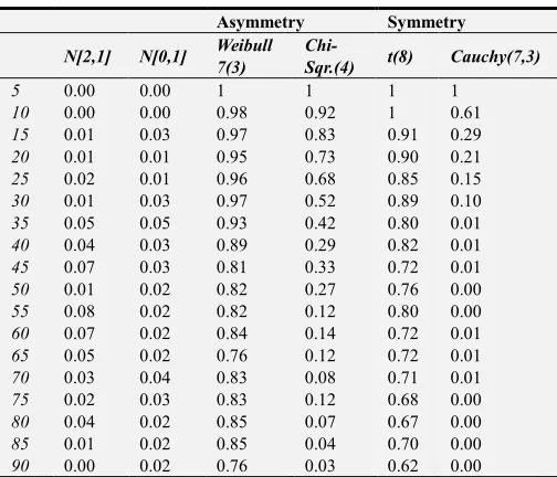
Table 5. Error Rate of Lilliefor’s Test Statistic.
Asymmetry Symmetry
N[2,1] N[0,1] Weibull 7(3)
Chi-Sqr.(4) t(8) Cauchy(7,3) 5 0.08 0.06 0.96 0.94 0.93 0.67 10 0.06 0.06 0.95 0.83 1 0.46 15 0.04 0.05 0.97 0.76 0.90 0.20 20 0.02 0.01 0.91 0.69 0.96 0.18 25 0.03 0.02 0.89 0.67 0.89 0.11 30 0.02 0.04 0.92 0.52 0.86 0.08 35 0.02 0.04 0.89 0.46 0.94 0.02 40 0.03 0.04 0.93 0.41 0.94 0.01 45 0.03 0.03 0.89 0.44 0.88 0.01 50 0.04 0.03 0.85 0.31 0.88 0.00 55 0.02 0.02 0.82 0.25 0.91 0.00 60 0.02 0.03 0.81 0.24 0.83 0.01 65 0.02 0.03 0.79 0.25 0.93 0.01 70 0.01 0.04 0.80 0.10 0.86 0.01 75 0.02 0.03 0.86 0.10 0.88 0.00 80 0.02 0.05 0.85 0.08 0.90 0.00 85 0.01 0.04 0.93 0.10 0.87 0.00 90 0.02 0.04 0.75 0.03 0.85 0.00 95 0.02 0.04 0.82 0.03 0.83 0.00 100 0.01 0.03 0.79 0.04 0.81 0.00
Lilliefors’ test statistic has lower sensitivity, an indication that the test statistic is weak in test of normality except Cauchy (7, 3).
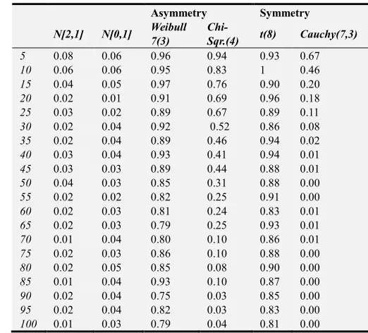
Table 6. Error Rates of Shapiro-Wilk Test Statistic.
Asymmetry Symmetry
N[2,1] N[0,1] Weibull 7(3)
From Table 6, the error rate decreases as sample size increases, an indication of higher sensitivity for large sample sizes.
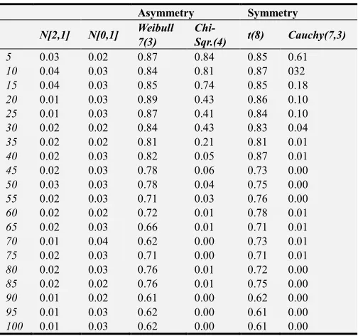
Table 7. Error Rate of Shapiro-Francia Test Statistic.
Asymmetry Symmetry
N[2,1] N[0,1] Weibull 7(3)
Chi-Sqr.(4) t(8) Cauchy(7,3) 5 0.03 0.02 0.87 0.84 0.85 0.61 10 0.04 0.03 0.84 0.81 0.87 032 15 0.04 0.03 0.85 0.74 0.85 0.18 20 0.01 0.03 0.89 0.43 0.86 0.10 25 0.01 0.03 0.87 0.41 0.84 0.10 30 0.02 0.02 0.84 0.43 0.83 0.04 35 0.02 0.02 0.81 0.21 0.81 0.01 40 0.02 0.03 0.82 0.05 0.87 0.01 45 0.02 0.03 0.78 0.06 0.73 0.00 50 0.03 0.03 0.78 0.04 0.75 0.00 55 0.02 0.03 0.71 0.03 0.76 0.00 60 0.02 0.02 0.72 0.01 0.78 0.01 65 0.02 0.03 0.66 0.01 0.71 0.01 70 0.01 0.04 0.62 0.00 0.73 0.01 75 0.02 0.03 0.71 0.00 0.71 0.01 80 0.02 0.03 0.76 0.01 0.72 0.00 85 0.02 0.02 0.76 0.01 0.75 0.00 90 0.01 0.02 0.61 0.00 0.62 0.00 95 0.01 0.03 0.62 0.00 0.61 0.00 100 0.01 0.03 0.62 0.00 0.61 0.00
The Shapiro-Francia has decreasing error rates as sample size increases. When compared with Shapiro-Wilk, it also has lower error rates, which makes it better than Shapiro-Wilk test statistic.
Table 8. Error Rate of Ryan-Joiner Test Statistic.
Asymmetry Symmetry
N[2,1] N[0,1] Weibull 7(3)
Chi-Sqr.(4) t(8) Cauchy(7,3) 5 0.06 0.05 0.06 0.09 0.19 0.75 10 0.03 0.05 0.05 0.18 0.19 0.65 15 0.03 0.03 0.06 0.28 0.18 0.43 20 0.04 0.05 0.06 0.24 0.11 0.32 25 0.02 0.05 0.06 0.31 0.17 0.21 30 0.05 0.05 0.06 0.47 0.19 0.11 35 0.05 0.03 0.08 0.76 0.09 0.08 40 0.04 0.02 0.12 0.73 0.72 0.04 45 0.05 0.03 0.13 0.75 0.70 0.02 50 0.02 0.03 0.10 0.73 0.81 0.00 55 0.05 0.04 0.12 0.81 0.78 0.01 60 0.08 0.04 0.17 0.84 0.78 0.01 65 0.03 0.04 0.18 0.83 0.69 0.01
Asymmetry Symmetry
N[2,1] N[0,1] Weibull 7(3)
Chi-Sqr.(4) t(8) Cauchy(7,3) 70 0.03 0.03 0.10 0.83 0.57 0.01 75 0.03 0.03 0.10 0.83 0.43 0.00 80 0.04 0.02 0.18 0.91 0.55 0.00 85 0.02 0.02 0.16 0.92 0.55 0.00 90 0.02 0.03 0.16 0.91 0.40 0.00 95 0.02 0.02 0.21 0.93 0.52 0.00 100 0.02 0.02 0.21 0.94 0.35 0.00
From Table 8, Ryan-Joiner test statistic is good for small sample sizes but poor for large sample sizes except Cauchy and normal distributions.
Table 9. Error Rate of Anderson Darling Test Statistic.
Asymmetry Symmetry
N[2,1] N[0,1] Weibull 7(3)
Chi-Sqr.(4) t(8) Cauchy(7,3)
5 0.00 0.00 0.99 1 1 1
10 0.00 0.00 0.98 0.98 0.92 0.77 15 0.01 0.03 0.98 0.97 0.92 0.31 20 0.01 0.01 0.9 0.87 0.90 0.22 25 0.02 0.01 0.9 0.82 0.88 0.14 30 0.01 0.03 0.96 0.73 0.76 0.11 35 0.05 0.04 0.93 0.44 0.79 0.05 40 0.04 0.03 0.85 0.31 0.80 0.04 45 0.04 0.03 0.83 0.30 0.73 0.05 50 0.01 0.02 0.83 0.31 0.72 0.02 55 0.05 0.02 0.82 0.29 0.76 0.01 60 0.05 0.02 0.83 0.21 0.72 0.01 65 0.05 0.02 0.75 0.20 0.72 0.01 70 0.03 0.02 0.76 0.09 0.70 0.01 75 0.02 0.03 0.72 0.10 0.69 0.01 80 0.03 0.02 0.78 0.06 0.69 0.00 85 0.01 0.01 0.77 0.03 0.70 0.00 90 0.00 0.01 0.76 0.03 0.62 0.00 95 0.00 0.02 0.73 0.01 0.62 0.00 100 0.01 0.02 0.71 0.00 0.42 0.00
The error rates show that Anderson Darling’s test statistic is good for small sample sizes but poor for large sample sizes except for Cauchy and normal distributions. See Table 10 for power of the nine methods considered.
9. Power of Test
Table 10. Power of Nine Selected Univariate Normality Tests Under Evaluation.
5 10 15 20 25 30 35 40 45 50 55 60 65 70 75 80 85 90 95 100
Weibull (7,3) 0.09 0.12 0.09 0.18 0.12 0.13 0.08 0.09 0.11 0.12 0.14 0.24 0.22 0.16 0.25 0.21 0.27 0.23 0.22 0.26 W/S Chi-Sqr (4) 0.14 0.03 0.09 0.06 0.19 0.15 0.15 0.18 0.1 0.22 0.22 0.21 0.19 0.17 0.24 0.23 0.24 0.22 0.21 0.18 t(8) 0.09 0.11 0.2 0.21 0.24 0.15 0.23 0.22 0.35 0.24 0.21 0.3 0.29 0.27 0.34 0.31 0.35 0.36 0.4 0.38 Cauchy (7,3) 0.08 0.29 0.52 0.75 0.83 0.86 0.92 0.96 0.96 0.99 0.99 0.99 0.99 0.98 1 0.99 1 1 1 1 Weibull (7,3) 0 0.02 0.03 0.05 0.04 0.03 0.07 0.11 0.19 0.18 0.18 0.16 0.24 0.17 0.17 0.15 0.15 0.24 0.3 0.3 JB Chi-Sqr (4) 0 0.08 0.17 0.27 0.32 0.48 0.58 0.71 0.67 0.73 0.88 0.86 0.88 0.92 0.88 0.93 0.96 0.97 1 1
5 10 15 20 25 30 35 40 45 50 55 60 65 70 75 80 85 90 95 100
Weibull (7,3) 0.97 0.95 0.93 0.94 0.94 0.96 0.88 0.86 0.77 0.8 0.78 0.83 0.72 0.8 0.8 0.82 0.84 0.74 0.69 0.69 AJB Chi-Sqr (4) 0.96 0.83 0.76 0.65 0.63 0.47 0.39 0.27 0.25 0.27 0.11 0.1 0.11 0.07 0.12 0.06 0.04 0.03 0 0
t(8) 0.93 0.95 0.89 0.87 0.82 0.86 0.77 0.18 0.3 0.29 0.32 0.32 0.31 0.33 0.37 0.35 0.35 0.4 0.38 0.45 Cauchy (7,3) 0.29 0.59 0.82 0.84 0.9 0.91 0.99 1 0.99 1 1 0.99 0.99 0.99 1 1 1 1 1 1 Weibull (7,3) - 0.47 0.47 0.48 0.48 0.49 0.58 0.57 0.68 0.68 0.68 0.64 0.78 0.77 0.79 0.79 0.81 0.79 0.78 0.8 D'Agostino Chi-Sqr (4) - 0.36 0.41 0.29 0.32 0.49 0.66 0.58 0.64 0.59 0.64 0.53 0.69 0.74 0.79 0.77 0.74 0.82 0.79 0.82
t(8) - 0.27 0.28 0.26 0.27 0.22 0.26 0.38 0.36 0.37 0.38 0.35 0.38 0.39 0.36 0.34 0.38 0.35 0.38 0.38 Cauchy (7,3) - 0.85 0.82 0.85 0.87 0.89 0.91 0.94 0.95 0.98 0.98 0.99 0.99 0.99 0.99 1 0.99 1 1 1 Weibull (7,3) 0.04 0.05 0.03 0.09 0.11 0.08 0.11 0.07 0.11 0.15 0.18 0.19 0.21 0.2 0.14 0.15 0.07 0.25 0.18 0.21 Lilliefor's Chi-Sqr (4) 0.06 0.17 0.24 0.31 0.33 0.48 0.54 0.59 0.56 0.69 0.75 0.76 0.75 0.9 0.9 0.92 0.9 0.97 0.97 0.96 t(8) 0.07 0 0.1 0.04 0.11 0.14 0.06 0.06 0.12 0.12 0.09 0.17 0.07 0.14 0.12 0.1 0.13 0.15 0.17 0.19 Cauchy (7,3) 0.33 0.54 0.8 0.82 0.89 0.92 0.98 0.99 0.99 1 1 0.99 0.99 0.99 1 1 1 1 1 1 Weibull (7,3) 0.03 0.09 0.04 0.11 0.1 0.2 0.15 0.14 0.26 0.24 0.27 0.21 0.33 0.32 0.26 0.2 0.18 0.37 0.34 0.33 SW Chi-Sqr (4) 0.05 0.18 0.38 0.43 0.58 0.67 0.79 0.91 0.93 0.93 0.96 1 0.99 1 1 0.99 0.99 1 1 1 t(8) 0.12 0.01 0.13 0.11 0.13 0.14 0.15 0.1 0.23 0.22 0.2 0.18 0.24 0.26 0.3 0.27 0.22 0.33 0.35 0.35 Cauchy (7,3) 0.29 0.56 0.78 0.87 0.9 0.95 1 1 0.99 1 1 0.99 0.99 0.99 1 1 1 1 1 1 Weibull (7,3) 0.13 0.16 0.15 0.11 0.13 0.16 0.19 0.18 0.22 0.22 0.29 0.28 0.34 0.38 0.29 0.24 0.24 0.39 0.38 0.38 SF Chi-Sqr (4) 0.16 0.19 0.26 0.57 0.59 0.57 0.79 0.95 0.94 0.96 0.97 0.99 0.99 1 1 0.99 0.99 1 1 1 t(8) 0.15 0.13 0.15 0.14 0.16 0.17 0.19 0.13 0.27 0.25 0.24 0.22 0.29 0.27 0.29 0.28 0.25 0.38 0.39 0.39 Cauchy (7,3) 0.39 0.68 0.82 0.9 0.9 0.96 0.99 0.99 1 1 1 0.99 0.99 0.99 0.99 1 1 1 1 1 Weibull (7,3) 0.94 0.95 0.94 0.94 0.94 0.94 0.92 0.88 0.87 0.9 0.88 0.83 0.82 0.9 0.9 0.82 0.84 0.84 0.79 0.79 RJ Chi-Sqr (4) 0.91 0.82 0.72 0.76 0.69 0.53 0.24 0.27 0.25 0.27 0.19 0.16 0.17 0.17 0.17 0.09 0.08 0.09 0.07 0.06
t(8)
Cauchy (7,3) 0.81 0.25
0.81 0.35
0.82 0.57
0.89 0.68
0.83 0.79
0.81 0.89
0.91 0.92
0.28 0.96
0.3 0.98
0.19 1
0.22 0.99
0.22 0.99
0.31 0.99
0.43 0.99
0.57 1
0.45 1
0.45 1
0.6 1
0.48 1
0.65 1 Weibull (7,3) 0.01 0.02 0.02 0.1 0.1 0.04 0.07 0.15 0.17 0.17 0.18 0.17 0.25 0.24 0.28 0.22 0.23 0.24 0.27 0.29 AD Chi-Sqr (4) 0.00 0.02 0.03 0.13 0.18 0.27 0.56 0.69 0.7 0.69 0.71 0.79 0.8 0.91 0.9 0.94 0.97 0.97 0.99 1
t(8) Cauchy (7,3)
0.00 0.00
0.08 0.29
0.08 0.69
0.10 0.79
0.12 0.86
0.24 0.89
0.21 0.95
0.20 0.96
0.27 0.95
0.28 0.98
0.24 0.99
0.28 0.99
0.28 0.99
0.30 0.99
0.31 0.99
0.31 1
0.30 1
0.38 1
0.38 1
0.58 1
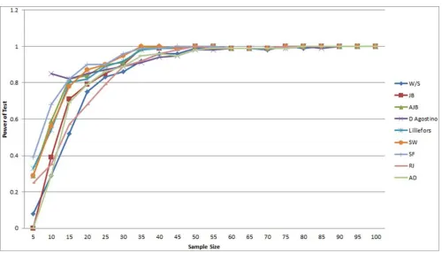
A test statistic with higher power is better, hence, the higher the power of a method, the better is the method. From Table 3.2, it can be seen that as the sample size increases, the power of normality tests increase, collaborating the findings of researchers like; Stephen (1974), Douglas and Edith (2002), Siddik (2006), Derya et al (2006), Frain (2006), Nor-Aishah and Shamsul (2007), Rinnakorn and Kamon (2007), Zvi et al (2008), Nornadiah and Yap (2011), Yap and Sim (2011), and Shigekazu et al (2012). The superiority of the method is easier visualised from graph of the power of the tests against sample sizes, see Figures 1 and 2.
Comparison of Power of the Test Statistics Using Line Chart
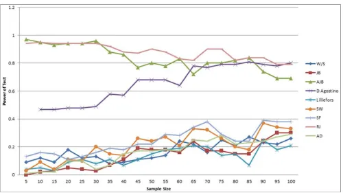
Figure 2. Power of Test using Weibull Distribution (Asymmetric Distribution).
From Figure 1, D’Agostino test statistic has highest power for a sample size of 10 while Shapiro-Francia test statistic has highest power for sample size 5 to 30 (except when n = 10). For sample size 35 and above, Shapiro-Francia has equal power as Shapiro-Wilk test statistic. It can also be seen that the best method for small sample size is not the best method for large sample size and that as the sample size increases, the power of the tests became unilateral/uniform.
From Figure 2, it can be deduced that Adjusted Jarque-Bera, Ryan-Joiner and D’Agostino tests have the highest power for asymmetric distributions irrespective of sample size. Other techniques have considerably and consistently low power for both small and large sample sizes.
Using both type I error and power of test, the ranking of the considered normality tests is as shown in Table 3.3;
Table 11. Normality Tests in Order of Superiority by Sample Sizes using Power of Test and Type I Error.
Sample Size
Order of Superiority of normality tests
1st 2nd 3rd 4th 5th 6th 7th 8th 9th
5 AJB Lf RJ SW SF W/S AD JB DA 10 AJB Lf DA RJ SF SW W/S JB AD 15 AJB Lf DA RJ SF SW JB W/S AD 20 AJB Lf DA RJ SF SW AD JB W/S 25 AJB Lf DA RJ SF SW W/S JB AD 30 AJB Lf DA SF RJ SW JB AD W/S 35 AJB Lf DA RJ SF JB AD SW W/S 40 DA Lf AJB RJ SF AD JB SW W/S 45 DA RJ SF Lf AJB JB AD SW W/S 50 DA RJ SF AJB Lf JB AD SW W/S 55 DA RJ SF Lf JB AJB AD SW W/S 60 DA RJ SF JB AJB AD Lf SW W/S
Sample Size
Order of Superiority of normality tests
1st 2nd 3rd 4th 5th 6th 7th 8th 9th
65 DA RJ SF JB AD Lf AJB SW W/S 70 DA RJ SF Lf JB AD SW AJB W/S 75 DA Lf RJ SF AD JB AJB SW W/S 80 DA RJ AD SF JB Lf AJB SW W/S 85 DA AD RJ JB SF Lf AJB SW W/S 90 DA RJ SF JB AD Lf SW AJB W/S 95 DA RJ SF JB AD Lf SW AJB W/S 100 DA AD RJ JB SF Lf SW AJB W/S
10. Conclusion
From all the results obtained from this study, we conclude as follows;
1. For small sample data, n≤30, the best three normality techniques in order of superiority are; (i) Adjusted Jaque-Bera test (ii) Lilliefor’s test and (iii) D’Agostino test. 2. For large sample data, n>30, the best three normality
techniques in order of superiority are; (i) D’Agostino test (ii) Ryan-Joiner test and (iii) Shapiro-Francia test. Thus, D’Agostino test is one of the best methods for small sample sizes, as well as large sample sizes, thus, it can be referred to as Uniformly Most Powerful amongst of all the tests evaluated.
3. The Adjusted Jarque-Bera (AJB) is consistently better than Jarque-Bera (JB) for sample data of size n≤50 while for n>50, JB is better, thus, the AJB should be used for small sample while JB should be used for large sample. This finding validates the purpose of modification of JB (Urzua, 1996).
Shapiro-Wilk (SW) for small and large sample data, hence, the SW should be replaced by SF in normality test. This contradicts the claims of researchers such as Yap and Sim (2011), Nor-Aisha et al (2011), Marmolejo-Ramos and Gonza’Lez-Burgos (2012), and Mayette (2013) that Shapiro-Wilk test statistic is the best method without consideration of SF.
5.W/S test is the worst amongst all the normality testing procedures; hence, it should be removed from the list of normality tests or adjusted for improved efficiency. We recommend as follows;
D’Agostino test statistic can be referred to as Uniformly Most Powerful among considered methods. Shapiro-Francia is a true improved method over SW for all sample sizes, hence, SF should replace SW. Proper modification of W/S to improve its sensitivity is very necessary, otherwise, W/S should be removed from the list of normality test statistics. D’Agostino D can be compared with other existing normality techniques not considered in this work for further validation of its superiority.
References
[1] Abbas M. (2013): Robust Goodness of Fit Test Based on the Forward Search. American Journal of App. Mathematics and Statistics, 2013, Vol. 1, No. 1, 6-10.
[2] Anderson, T. W. (1962): On the Distribution of the Two-Sample Cramer–von Mises Criterion. The Annals of Mathematical Statistics (Institute of Mathematical Statistics) 33 (3): 1148–1159. doi:10.1214/aoms/1177704477. ISSN 0003-4851.
[3] Baghban A. A., Younespour S., Jambarsang S., Yousefi M., Zayeri F., and Jalilian F. A. (2013): How to test normality distribution for a variable: a real example and a simulation study. Journal of Paramedical Sciences (JPS). Vol.4, No.1 ISSN 2008-4978.
[4] D’Agostino R. B. and Stephens M. A. (1986): Goodness-of-fit techniques. New York, Marcel Dekker.
[5] Derya O., Atilla H. E., and Ersoz T. (2006): Investigation of Four Different Normality Tests in Terms of Type I Error Rate and Power Under Different Distributions. Turk. J. Med. Sci. 2006; 36 (3): 171-176.
[6] Douglas G. B. and Edith S. (2002): A test of normality with high uniform power. Journal of Computational Statistics and Data Analysis 40 (2002) 435–445.
www.elsevier.com/locate/csda.
[7] Everitt, B. S. (2006): The Cambridge Dictionary of Statistics. Third Edition. Cambridge University Press, Cambridge, New York, Melbourne, Madrid, Cape Town, Singapore, Sao Paulo. Pp. 240-241.
[8] Farrel P. J and Stewart K. R. (2006): Comprehensive Study of Tests for Normality and Symmetry; Extending the Spiegelhalter Test. Journal of Statistical Computation and Simulation. Vol. 76, No. 9, Pp 803-816.
[9] Frain J. C. (2006): Small Sample Power of Tests of Normality when the Alternative is an α -stable
distribution.http://www.tcd.ie/Economics/staff/frainj/Stable_D istribution/normal.pdf
[10] Guner B. and Johnson J. T. (2007): Comparison of the Shapiro-Wilk and Kurtosis Tests for the Detection of Pulsed Sinusoidal Radio Frequency Interference. The Ohio State University, Department of Electrical and Computer Engineering and Electro-Science Laboratory, 1320 Kinnear Road, Columbus, OH 43210, USA.
[11] Gupta S. C. (2011): Fundamentals of Statistics. Sixth Revised and Enlarged Edition. Himilaya Publishing House PVT Ltd. Mumbai-400 004. Pp 16. 28-16.31
[12] Jarque, C. M. and Bera, A. K. (1980): Efficient tests for normality, homoscedasticity and serial independence of regression residuals. Economics Letters 6 (3): 255–259. doi:10.1016/0165-1765(80)90024-5.
[13] Jarque, C. M. and Bera, A. K. (1981): Efficient tests for normality, homoscedasticity and serial independence of regression residuals: Monte Carlo evidence. Economics Letters 7 (4): 313–318. doi:10.1016/0165-1765(81)900235-5. [14] Jarque, C. M. and Bera, A. K. (1987): A test for normality of
observations and regression residuals. International Statistical Review 55 (2): 163–172. JSTOR 1403192.
[15] Jason O. (2002): Notes on the use of data transformations. Practical Assessment, Research & Evaluation, 8(6). http://PAREonline.net/getvn.asp?v=8&n=6.
[16] Jason O. (2010): Improving your data transformations: Applying the Box-Cox transformation. Practical Assessment, Research & Evaluation, 15(12). Available online: http://pareonline.net/getvn.asp?v=15&n=12.
[17] Marmolejo-Ramos F. and Gonza´lez-Burgos J. (2012): A Power Comparison of Various Tests of Univariate Normality on Ex-Gaussian Distributions. European Journal of Research Methods for the Behavioural and Social Sciences. ISSN-Print 1614-1881· ISSN-Online 1614-2241. DOI: 10.1027/1614-2241/a000059. www.hogrefe.com/journals/methodology [18] Mayette S. and Emily A. B. (2013): Empirical Power
Comparison of Goodness of Fit Tests for Normality in the Presence of Outliers. Journal of Physics. Conference Series 435 (2013) 012041.doi:10.1088/1742-6596/435/1/012041. [19] Molin P. and Abdi H. (2007): Lilliefors/Van Soest’s test of
normality. Encyclopedia of measurement and Statistics. Pp. 1-10. www.utd.edu/~herve
[20] Narges A. (2013): Shapiro-Wilk Test in Evaluation of Asymptotic Distribution on Estimators of Measure of Kurtosis and Skew. International Mathematical Forum, Vol. 8, 2013, no. 12, 573–576. HIKARI Ltd, www.m-hikari.com
[21] Nor A. A, Teh S. Y., Abdul-Rahman O. and Che-Rohani Y. (2011): Sensitivity of Normality Tests to Non-Normal Data. Sains Malaysiana 40 (6) (2011): 637–641.
[22] Nor-Aishah H. and Shamsul R. A (2007): Robust Jacque-Bera Test of Normality. Proceedings of The 9th Islamic Countries Conference on Statistical Sciences 2007. ICCS-IX 12-14 Dec 2007
[24] Panagiotis M. (2010): Three Different Measures of Sample Skewness and Kurtosis and their Effects on the Jarque-Bera Test for Normality. Jonkoping International Business School Jönköping University JIBS, Sweden. Working Papers No. 2010-9.
[25] Piegorsch W. W and Bailer A. J. (2005): Analyzing Environmental Data. Page: 432. John Wiley & Sons, Ltd. The Atrian, South Gate, Chichester, West Sussex P019 85Q, England. ISBN: 0-470-84836-7 (HB).
[26] Pitchaya S., Dee A. B., and Kevin S. (2012): Exploring the Impact of Normality and Significance Tests in Architecture Experiments. Department of Computer Science, University of Virginia.
[27] Richard M. F. and Ciriaco V. F. (2010): Applied Probability and Stochastic Processes. Springer Heidelberg Dordrecht, London New York. Pp 95-96. ISBN: 978-3-642-05155-5. DOI: 10.1007/978-3-642-05158-6
[28] Rinnakorn C., and Kamon B. (2007): A Power Comparison of Goodness-of-fit Tests for Normality Based on the Likelihood Ratio and the Non-likelihood Ratio. Thailand Statistician, July 2007; 5: 57-68. http://statassoc.or.th.
[29] Royston J. P (1983): A Simple Method for Evaluating the Shapiro-Francia W' Test of Non-Normality. Journal of the Royal Statistical Society. Series D (The Statistician), Vol. 32,
No. 3 (Sep.,1983), pp. 297-300.
http://www.jstor.org/stable/2987935. Accessed: 26/07/2014. [30] Ryan, T. A. and Joiner B. L. (1976): Normal Probability Plots
and Tests for Normality, Technical Report, Statistics Department, The Pennsylvania State University.
[31] Ryan T. A. and Joiner B. L. (1990): Normal probability plots and tests for normality. Minitab Statistical Software: Technical Reports, November, 1-14.
[32] Schaffer M. (2010): Procedure for Monte Carlo Simulation. SGPE QM Lab 3. Monte Carlos Mark version of 4.10.2010.
[33] Seth R. (2008): Transform your data; Statistics column. Nutrition 24, Pp 492–494. Elsevier. doi:10.1016/j.nut.2008.01.00
[34] Shigekazu N., Hiroki H. and Naoto N. (2012): A Measure of Skewness for Testing Departures from Normality. Journal of Computational Statistics and Data Analysis. XIV: 1202.5093V1.
[35] Siddik K. (2006): Comparison of Several Univariate Normality Tests Regarding Type I Error Rate and Power of the Test in Simulation based Small Samples Journal of Applied Science Research 2 (5): 296-300, 2006. © 2006, INSInet Publication.
[36] Stephen M. A (1974): EDF Statistics for Goodness of Fit and Some Comparisons. Journal of the American Statistical Association. Theories and Methods Section, Vol. 69, No 347, Pp 730-737. http://www.jstor.org.
[37] Urzúa, C. M. (1996): On the correct use of omnibus tests for normality, Economics Letters 53: 247-251. http://www.sciencedirect.com/science/article/pii/S0165176596 009238
[38] Weurtz, D. and Katzgraber H. G (2005). Precise finite-sample quantiles of the Jarque-Bera adjusted Lagrange multiplier test. Swiss Federal Institute of Technology, Institute for Theoretical Physics, ETH H¨onggerberg, C-8093 Zurich.
[39] Yap B. W. and Sim C. H. (2011): Comparisons of various types of normality tests. Journal of Statistical Computation
and Simulation 81:12, 2141-2155,
DOI:10.1080/00949655.2010.520163.