Page | 10
Extended Spectral Nonlinear Conjugate Gradient
methods for solving unconstrained problems
Dr. Basim A. Hassan
Asst. Professor, College of Computers Sciences and Math., University of Mosul, Iraq
ABSTRACT
In this paper, we present extension forms of Dai, Yuan (DY), Fletcher, Reveres (FR) and Conjugate Descent (CD) CG algorithms. The extended method have the sufficient descent and globally convergence properties under certain conditions. These new algorithms are tested on some standard test functions and compared with the original FR algorithm showing considerable improvements over all these comparisons.
Keywords: Conjugate gradient method, Spectral Conjugate gradient method, sufficient descent property, global convergent methods.
INTRODUCTION
The nonlinear conjugate gradient (CG) method is designed to solve the following unconstrained optimization problem
min
f
(
x
)
x
R
n
...
(
1
)
where
f
:
R
n
R
is a continuously differentiable nonlinear function whose gradient is denoted byg
. Due to its simplicity and its very low memory requirement, the CG method has played a special role for solving large scale nonlinear optimization problems. The iterative formula of the CG method is given by
x
k1
x
k
kd
k...
(
2
)
where
k
0
is a step length which is computed by carrying out a line search and satisfies the standard Wolfe (SW ) conditions :
f
(
x
k
kd
k)
f
(
x
k)
1
kd
kTg
k...
(
3
)
g
(
x
k
kd
k)
Td
k
2d
kTg
k...
(
4
)
with0
1
2
1
, andd
k1 is the search direction defined by
,
1
,
1
1 1 1
k
d
g
k
g
d
k k k
k
...
(
5
)
where
d
k is a descent direction. Different conjugate gradient algorithms correspond to different choices for the scalar parameter
ksee [7]. The well-known formula of
k are given by,
1 1
k T k
k T k FR k
g
g
g
g
...
(
6
)
,
1 1
k T k k T k CD k
d
g
g
g
...
(
7
)
,
1 1
k T k
k T k DY k
d
y
g
g
...
(
8
a
)
Page | 11
k T k
k T k DY k
d
g
d
g
1 1
....
(
8
b
)
In [6] modified conjugate gradient methods are given by the rule
k k k
k k T k k
k
g
d
g
d
g
d
2 1
1 1
1
1
...
(
9
)
where
k is one of the values in(
6
)
or(
7
)
or(
8
)
.Zhang and Wang [8] proposed a general form of conjugate gradient methods are given by the rule
k k k
k k T k k
k
g
d
g
d
y
d
2 1
1
1
...
(
10
)
where
k is one of the values in(
6
)
or(
7
)
or(
8
)
.The paper is organized as follows. In section (1) is the introduction. In section (2) we present the extended spectral method and algorithm. Section (3) show that the search direction generated by this proposed algorithm at each iteration satisfies the sufficient descent condition and establishes the global convergence analysis. Section (4) establishes some numerical results to show the effectiveness of the proposed CG-method and Section (5) gives a brief conclusions .
Extended spectral conjugate gradient method and algorithm
In this paper we suggest a new type of spectral conjugate gradient methods for solution of the
min
f
(
x
)
. In [5] we consider a condition that a descent search direction is generated, and we extend the DY method. We make such a direction inductively. Suppose that the current search directiond
k is a descent direction, namely,g
kTd
k
0
at theth
k
iteration. Now we need to find a
k that produces a descent search directiond
k1. This requires thatk T k k k
k T
k
d
g
g
d
g
1 1
1 2
1 ....
(
11
)
Letting
k1 be a positive parameter, we define1 2 1
k k k
g
....
(
12
)
Equation
(
11
)
is equivalent tok T k k1
g
1d
....
(
13
)
Taking the positively of
k1 in to consideration, we have
,
0
max
11 k
T k k
g
d
....
(
14
)
Therefore if condition
(
14
)
is satisfied for allk
,
the conjugate gradient method with(
12
)
produces a descent search direction at every iteration. From(
12
)
we can get various kinds of conjugate gradient method by choosing various1 k
.Hideaki and Yasushi proposed a new conjugate gradient method which was obtained by modifying the DY method and called MDY method. A nice property of the MDY method is that it generates sufficient descent directions. The parameter
k in MDY method is given by1 1 1
k k T k MDY k
g
g
...
(
15
)
where
)
(
2
1
1
k
k kk
f
f
...
(
16
)
Page | 12
,
)
(
1 11 2
1 1
1
MDY k k T k k k
T k MDY k k
k T
k
d
g
g
d
g
d
g
...
(
17
)
and hence,
k k k
T k
k T k k
T k k
k T k k
d
g
d
g
d
g
d
g
1 1 11 1
1 1
0
....
(
18
)
performs more effective More details can be found in [5].
Let us try to derive a new type method we need the next direction
d
k1 to be descent. Assume that
k
0
. By this, we have for any
(
0
,
1
]
, and from(
13
)
the following inequality holds :,
1 2
1 1
1 1
k T k k k
k k
k T k k k k
d
g
g
d
g
)
19
(
...
i.e. ,
0
1 1
2
1
kT k k k k
k
g
d
g
....
(
20
)
Now we can rewrite the above inequality as
0
1 2 1
1
1
k k k
k k k T
k
g
d
g
g
....
(
21
)
Hence, we obtain our new directions as follows :
k k k k
k k
k
g
d
g
d
2 1
1 1
1 .
...
(
22
)
Then we can rewrite
(
22
)
ask k k k
k
g
d
d
1
1
....
(
23
)
where
2 1
1
k k k k
g
....
(
24
)
This method includes the Zhang and Wang (ZW) method as a special case. By setting
k1
y
kTd
k,
direction(
22
)
reduces to the Zhang and Wang (ZW) method which defined in(
10
)
.Now we can obtain the a new conjugate gradient algorithms, as follows : The New Algorithm (2.1)
Step 1. Initialization : Select
x
1
R
n and the parameters0
1
2
1
. Computef
(
x
1)
andg
1. Considerd
1
g
1 and set the initial guess
1
1
/
g
1 .Step 2. Test for continuation of iterations. If
g
k1
10
6, then stop. else step3.Step 3. Line search : Compute
k1
0
satisfying the Wolfe line search condition (6) and update the variablesx
k1
x
k
kd
k.Step 4. Conjugate gradient parameter which defined in
(
6
)
or(
7
)
or(
8
)
.Step 5. Direction computation
d
k1 which defined in(
22
)
.If the restart criterion of Powellg
Tk1g
k
0
.
2
g
k1 2, is satisfied, then setd
k1
g
k1 otherwise defined
k1
d
.GLOBAL CONVERGENCE
In this section, we establish convergence of the proposed method, the following assumptions for the objective function are needed.
Page | 13
i- The level set
L
x
R
nf
(
x
)
f
(
x
0)
is bounded.ii- In some neighborhood
U
ofL
,
f
(
x
)
is continuously differentiable and its gradient is Lipschitz continuous, namely, there exists a constant
0
such that.
,
,
)
(
)
(
x
1g
x
L
x
1x
x
1x
U
g
k
k
k
k
k k
...
(
25
)
Assumption 3.1 imply that there exists a positive constant
such that.
,
1
x
U
g
k
...
(
26
)
Here we have to present sufficient descent property.
Theorem 1
Let
x
k1 and
d
k1 be generated by(
2
)
and(
22
),
where
k satisfies Wolfe line search conditions, then holds of the sufficient descent property2 1 1
1
k
k Tk
d
c
g
g
....
(
27
)
Proof :
Then conclusion can be proved by induction. When
k
0
,
we haveg
0Td
0
g
0 2
0
.Suppose that k k 2 T
k
d
c
g
g
. From(
13
)
and(
22
)
we havek T k k k T k k k
k T k k k k k
k k k k
k k T
k k T k
d
g
d
g
g
d
g
g
d
g
g
g
d
g
1 1
2 1
1 1
2 1
1 2 1
1 1
1 1
)
28
(
...
.
2 1 2
1 1
1
k
k
k Tk
d
g
c
g
g
...
(
29
)
where
c
. Thus the theorem is proved.The following Lemma [9] is the result for general iterative methods : Lemma 1
Suppose that Assumption 2.2 is satisfied and consider any method with Eq.
(
2
),
where
k satisfies Eqs.(
11
)
and)
12
(
. Then,
1
2 1
2 1 1
)
(
i k
k T k
d
d
g
.
...
(
30
)
From the previous analysis, we can get the following global convergence result for new Algorithm.
Theorem 2
Suppose that Assumption (3.1) holds, and these methods have the satisfies sufficient descent condition with
c
. Then these method are globally convergent, one has0
inf
lim
1
k
k
g
or
1
2 1
2 1
1
)
(
k k
k T k
d
d
g
.
...
(
31
)
Proof :
Page | 14
d
0
g
0 andg
k1
1...
(
32
)
By squaring the two sides of(
22
)
and transferring and trimming, we get :1 1 2 1 1 2 1 2 2 1 1 2 2 2
1
2
k T k k k k k k k k k kk
d
g
g
g
g
d
d
....
(
33
)
Dividing the previous in equation by
2 1
1
)
(
d
kTg
k, we get :
2 1 1 1 1 2 1 1 2 1 2 2 1 1 2 1 1 2 2 2 1 1 2 1)
(
2
)
(
)
(
)
(
k k k k T k k T k k k k k k T k k k k T k kg
g
d
g
d
g
g
g
d
d
g
d
d
)
34
(
...
2 1 2 1 2 1 1 1 1 2 1 1 2 1 2 2 1 1 2 1 1 2 2 2 1 1 2 11
1
)
(
2
)
(
)
(
)
(
k k k k k k T k k T k k k k k k T k k k k T k kg
g
g
g
d
g
d
g
g
g
d
d
g
d
d
)
35
(
...
2 1 2 1 2 1 1 1 1 2 1 1 2 2 2 1 1 21
1
1
)
(
1
)
(
)
(
k k k k k k T k k T k k k k T k kg
g
g
g
d
g
d
d
g
d
d
)
36
(
...
2 1 2 1 1 2 2 2 1 1 2 11
)
(
)
(
k k T k k k k T k kg
g
d
d
g
d
d
)
37
(
...
a. When
k
kDY. Then by(
8
b
)
k T k k T k DY k
d
g
d
g
1 1
...
(
38
)
and applying
(
37
)
, we have2 1 2 2 2 1 1 2 1
1
)
(
)
(
k k T k k k T k kg
g
d
d
g
d
d
)
39
(
...
Noting that,
1
)
(
1 1 2 1 22 1
g
g
d
d
T
...
(
40
)
With this, from
(
32
)
we have2 1 1 1 2 1 2 1 1 2 1
1
)
(
k
g
g
d
d
k i i k T kk
.
...
(
41
)
Then we get
k
d
g
d
k k T k 2 1 2 1 2 1 1)
(
Page | 15 Which indicates
1 2 1 1 2 1 2 1 1)
(
k k k k T kk
d
g
d
.
...
(
43
)
This is a contradiction to the
(
30
)
.b. When
k
kFR. Then from(
37
)
and sufficient descent condition withc
.2 1 4 2 2 2 1 4 1 2 2 4 4 1 2 1 2 1 1 2 4 4 1 2 1 1 2 1
1
1
1
)
(
)
(
k k k k k k k k k k T k k k k k T k kg
g
c
d
g
g
c
d
g
g
g
g
d
d
g
g
g
d
d
)
45
(
...
we also have
1 2 1 1 2 1 2 1 1)
(
k k k k T kk
d
g
d
.c. When
k
kCD. Then from(
37
)
and sufficient descent condition withc
.2 1 4 4 2 2 1 4 1 2 2 4 2 4 1 2 1 2 1 1 2 2 4 1 2 1 1 2 1
1
1
1
)
(
)
(
)
(
k k k k k k k k k k T k k k T k k k T k kg
g
c
d
g
g
c
d
g
c
g
g
g
d
d
g
d
g
g
d
d
)
46
(
...
we also have
1 2 1 1 2 1 2 1 1)
(
k k k k T kk
d
g
d
.which contradicts Lemma 1. Therefore, we get this theorem.
NUMERICAL RESULTS
In this section, we will report the numerical performance of Algorithm (2.1). We test Algorithm (2.1) by solving the 15 benchmark problems from [1] and compare its numerical performance with that of the other similar method, which include the standard FR conjugate gradient method in [3]. All codes of the computer procedures are written in Fortran. The parameters are chosen as follows :
9
.
0
,
001
.
0
,
5
.
0
,
10
6
1
2
In Tables 1 and 2, we use the following denotations :
n : the dimension of the objective function. NOI : the number of iterations.
NOF : the number of function evaluations.
Page | 16
F : If NOF or NOI exceeded 2000 then denote F.
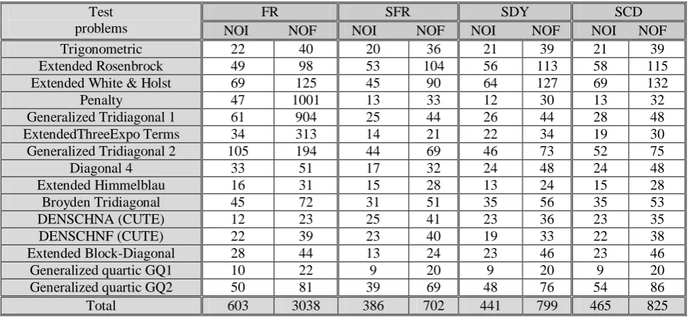
Table (4.1) Comparison of the algorithms for
n
100
Test problems
FR SFR SDY SCD
NOI NOF NOI NOF NOI NOF NOI NOF
Trigonometric 22 40 20 36 21 39 21 39
Extended Rosenbrock 49 98 53 104 56 113 58 115
Extended White & Holst 69 125 45 90 64 127 69 132
Penalty 47 1001 13 33 12 30 13 32
Generalized Tridiagonal 1 61 904 25 44 26 44 28 48
ExtendedThreeExpo Terms 34 313 14 21 22 34 19 30
Generalized Tridiagonal 2 105 194 44 69 46 73 52 75
Diagonal 4 33 51 17 32 24 48 24 48
Extended Himmelblau 16 31 15 28 13 24 15 28
Broyden Tridiagonal 45 72 31 51 35 56 35 53
DENSCHNA (CUTE) 12 23 25 41 23 36 23 35
DENSCHNF (CUTE) 22 39 23 40 19 33 22 38
Extended Block-Diagonal 28 44 13 24 23 46 23 46
Generalized quartic GQ1 10 22 9 20 9 20 9 20
Generalized quartic GQ2 50 81 39 69 48 76 54 86
Total 603 3038 386 702 441 799 465 825
Table (4.2) Comparison of the algorithms for
n
1000
Test problems
FR SFR SDY SCD
NOI NOF NOI NOF NOI NOF NOI NOF
Trigonometric 42 67 33 58 32 57 41 70
Extended Rosenbrock 60 113 65 126 61 122
Extended White & Holst 237 299 58 115 71 136 47 92
Penalty 26 209 16 43 12 30 13 37
Generalized Tridiagonal 1 43 390 30 57 58 993 39 376
ExtendedThreeExpo Terms 12 21 38 583 49 809
Generalized Tridiagonal 2 121 231 72 119 78 126 51 79
Diagonal 4 32 50 17 32 27 54 27 54
Extended Himmelblau 21 37 16 30 14 26 12 23
Broyden Tridiagonal 47 78 42 69 41 68 40 67
DENSCHNA (CUTE) 58 110 18 30 19 31 17 29
DENSCHNF (CUTE) 24 41 22 39 18 31 19 34
Extended Block-Diagonal 31 50 25 48 23 46 23 46
Generalized quartic GQ1 8 20 8 20 8 20 8 20
Generalized quartic GQ2 52 83 39 63 46 75 50 82
Total 742 1665 396 731 447 1247 387 1009
From the above numerical experiments, it is shown that the new algorithms in this paper is promising.
CONCLUSIONS AND DISCUSSIONS
In this paper, a new spectral conjugate gradient algorithm has been developed for solving unconstrained minimization problems. Under some mild conditions, the global convergence has been proved. Compared with the other similar algorithm, the numerical performance of the developed algorithm is promising.
Table (5.1) gives a comparison between the new-algorithm (2.1) and the Fletcher and Reeves (FR)-algorithm for convex optimization , this table indicates that the new algorithm (2.1) saves
(
58
66
)%
NOI and(
30
43
)%
Page | 17
Tools NOI NOF FR- algorithm 100 % 100 % SFR- algorithm 41.85 % 69.53 % SDY- algorithm 33.97 % 43.50 % SCD- algorithm 36.65 % 61.00 %
REFERENCES
[1]. Andrie, N. (2008) ' An Unconstrained Optimization Test functions collection' Advanced Modeling and optimization.10, pp.147-161.
[2]. Dai, Y. and Yuan Y. (1999) ' A nonlinear conjugate gradients method with a strong global convergence property' SIAM J. Optimization 10, pp.177-182.
[3]. Fletcher, R. (1987) ' Practical Methods of Optimization (second edition). John Wiley and Sons, New York. [4]. Fletcher, R. and Reeves C. (1964) ' Function minimization by conjugate gradients ' Computer J. 7, pp.149-154.
[5]. Hideaki I., Yasushi N., (2011). Conjugate gradient methods using value of objective function for unconstrained optimization Optimization Letters, V.6, Issue 5, 941-955.
[6]. Matonoha C., Luksan L. and Vlcek J. (2008) ' Computational experience with conjugate gradient methods for unconstrained optimization ' Technical report no.1038, pp.1-17.
[7]. Yabe H. and M. Takano, (2004). Global convergence properties of nonlinear conjugate gradient methods with modified secant condition, Comput. Optim. Appl., 28, 203–225.
[8]. Zhang Y. and Wang K. , (2012) ' A new general form of conjugate gradient methods with guaranteed descent and strong global convergence properties' , Numer Algor , 60, pp.135–152.
[9]. Zoutendijk, G. : Nonlinear programming. In: Abadie, J. (ed.) Integer and Nonlinear Programming, North-Holland, Amsterdam, 123, pp. 37–86.