Feng-temporal-coloring-MSWIM13.pdf

(1)

Algorithms for Channel Assignment in Mobile Wireless

Networks using Temporal Coloring

∗

Feng Yu

City University of New York Graduate Center New York, NY, 10016, USA

[email protected]

Amotz Bar-Noy

City University of New York

Graduate Center New York, NY, 10016, USA

[email protected]

Prithwish Basu

Raytheon BBN Technologies Cambridge, MA, 02138, USA

[email protected]

Ram Ramanathan

Raytheon BBN Technologies Cambridge, MA, 02138, USA

[email protected]

ABSTRACT

We model the problem of channel assignment in mobile networks as one oftemporal coloring(T-coloring), that is, coloring a time-varying graph. In order to capture the impact of channel re-assignments due to mobility, we model the cost of coloring asC+αA, where

Cis the total number of colors used andAis the total number of color changes, andαis a user-selectable parameter reflecting the relative penalty of channel usage and re-assignments.

Using these models, we present several novel algorithms for tem-poral coloring. We begin by analyzing two simple algorithms called SNAP and SMASH that take diametrically opposite positions on colors vs re-assignments, and provide theoretical results on the ranges ofαin which one outperforms the other, both for arbitrary and random time-varying graphs. We then present six more al-gorithms that build upon each of SNAP and SMASH in different ways. Simulations on random geometric graphs with random way-point mobility show that the relative cost of the algorithms depends upon the value ofαand the transmission range, and we identify precise values at which the crossovers happen.

Categories and Subject Descriptors

C.2.1 [Network Architecture and Design]: Wireless Communi-cation; G.2.2 [Graph Theory]: Graph algorithms

∗

Research was sponsored by the Army Research Laboratory and was ac-complished under Cooperative Agreement Number W911NF-09-2-0053. The views and conclusions contained in this document are those of the au-thors and should not be interpreted as representing the official policies, ei-ther expressed or implied, of the Army Research Laboratory or the U.S. Government. The U.S. Government is authorized to reproduce and dis-tribute reprints for Government purposes notwithstanding any copyright no-tation here on.

Permission to make digital or hard copies of all or part of this work for personal or classroom use is granted without fee provided that copies are not made or distributed for profit or commercial advantage and that copies bear this notice and the full cita-tion on the first page. Copyrights for components of this work owned by others than ACM must be honored. Abstracting with credit is permitted. To copy otherwise, or re-publish, to post on servers or to redistribute to lists, requires prior specific permission and/or a fee. Request permissions from [email protected].

Keywords

Channel Assignment; Mobile Wireless Networks; Graph Coloring; Random Graph; Time Varying Graph

1.

INTRODUCTION

The assignment ofchannelsto communicating nodes is a key part of contention-free medium access in a wireless network. De-pending upon the access method, the “channel" could be time slot [19], code [11] or frequency [9]. The problem also arises in multi-channel multi-radio cognitive networks where nodes opportunistically use a subset of a large number of unused frequencies [21].

Graph coloring is a natural model for channel assignment [10,15, 19]. It can capture several access methods such as TDMA, FDMA and CDMA in a unified way [18]. In this formulation, the vertices in the graph represent nodes in a multi-hop network, edges repre-sent links, and colors reprerepre-sent channels assigned to nodes. The coloring of the graph is typically done using constraints that reflect the application context. For example, for conflict-free slot assign-ment in TDMA one seeks to color the graphs using a minimum number of colors such that vertices within two hops (i.e., distance-2) of each other receive different colors, which in turn ensures that transmissions in two slots never collide.

Most of the work thus far on graph coloring has been onstatic

graphs. This does not capture networks where due to mobility or other link fluctuations, the network topology is varying over time. Applying static graph coloring to successive graph “snap-shots" does not capture properties that are validover time, for in-stance, a coloring that is conflict-free fortseconds in future. Fur-ther, the mismatch between the model (static graph) and the reality (mobile networks) is far from ideal.

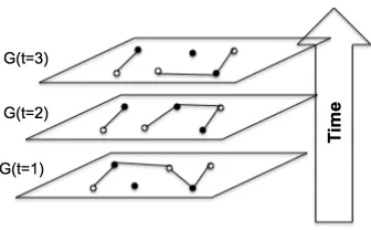
In this paper, we use a model that inherently captures dynamism, and hence mobility. Specifically, we model a network as a time-varying graphor temporal graph(T-graph). A T-graph is more than just a sequence of snapshots – it is a structure in and of itself that is manipulableas a whole, and for which properties can be definedacross time. For example, a “valid coloring" property can now be attributed to (an entire) temporal graph, e.g., a contiguous sub-sequence T-graph. One can also aggregate snapshots between arbitrary points in time to get new T-graphs, as detailed later. Figure 1 illustrates a time-varying graph with a conflict-free distance-1

(2)

Figure 1:Temporal Graphlets fort= 1,2,3, and a conflict-free tempo-ral coloring.

In static networks (graphs), the minimization criterion is typi-cally just the number of channels (colors) used. In a mobile net-work (temporal graph), however, there are two parameters of inter-est: the total number of colors used, and the number of times a node has to bere-assigneda color due to conflicts caused by mobility. In most real-life networks, a re-assignment of time slot or frequency requires the exchange of control packets which reduces data capac-ity. More crucially, it may cause packet drops since the distributed algorithms that implement a re-assignment of the channel take time to converge. Note that even the addition of a single edge can cause a network-wide ripple effect of re-coloring.

In general, the relative “cost" of total colors used and the ef-fect of re-coloring depends on the network system and its proto-cols. Accordingly, we use a generalized cost model where the cost of a dynamic coloring of a temporal graph is given byC+α.A

whereC is the total number of colors used, Ais the number of re-assignments over a period of timeTandαis a user-defined pa-rameter that “weights" the penalty of re-assignment relative to that of the total number of colors. For example, in a cognitive radio network where spectrum holes are plentiful,αwould be smaller than in a TDMA network where slots are precious. In Figure 1, for example,C= 2, A= 2.

We present several novel algorithms for coloring T-graphs (we call this T-coloring). We begin by taking two simple baseline al-gorithms that take extreme positions on the optimization function: SNAP, which colors each snapshot independently, and thus does not care about re-assignments at all; and SMASH, which takes the entire T-graph, “smashes" it into a single graph by taking the union of all edges, colors this graph, and uses the colors for the entire duration[1, T]. Thus, SMASH never re-assigns but makes little attempt to minimize total colors used. We then present six more sophisticated algorithms that enhance each of SNAP and SMASH in various ways, for example, by incrementally coloring or partially smashing. We evaluate the performance of several T-coloring algo-rithms using random geometric graph (RGG) and random waypoint mobility (RWP) models.

Our main contributions are as follows:

Temporal coloring and cost model. We present a new color-ing framework that captures mobility inherently. Our cost model

C+αAcaptures the relative impact of channel re-assignments and channels used in a user-selectable manner. Together, our frame-work better reflects real-world considerations.

Temporal coloring algorithms and analysis. We present a total of eight algorithms that cover a spectrum of strategies, including a hybrid one. We prove a number of properties on the relative perfor-mance of SNAP and SMASH. For example, we show that ifα >1 SMASH is always better than SNAP, and ifα= 0SNAP is never worse than SMASH, and for random graphs SNAP outperforms

SMASH w.h.p. ifα≤ 1 log 1

1−pn

for distance-1 coloring (we also

give an analogous result for distance-2 coloring). We also derive a network dynamics based threshold for a hybrid algorithm, based on the RGG-RWP model, that we then use for switching between two algorithms.

Insights from experiments.We present several experiments com-paring the algorithms and identify “pivot" points where pairs or triplets of algorithms reverse their relative performance. While no single algorithm is superior over the entire range ofα, our work provides insights to practitioners to choose the best algorithm for a given scenario.

Four of our eight algorithms require the entire T-graph in ad-vance and four do not. The former captures mobility or dynamism that are pre-defined (e.g. networks of aircraft or underwater nodes with pre-defined trajectories, scheduled sleep/wake sensor networks) or can be reasonably predicted somewhat into the future [24]. It is also applicable to dynamic job scheduling modeled as a coloring problem [1]. However, for simplicity and clarity, we assume in the description and in the experimental evaluation that all algorithms have the same input, namely the entire T-graph.

This paper follows the so-called "protocol model" for interfer-ence vice the SINR-based "physical model" [8]. While we recog-nize that the physical model is a better reflection of radio charac-teristics, our focus is on temporal aspects and a novel cost model. These are first better investigated in the simpler protocol model, with physical model extensions a topic for future work. Further, recent work [23] has shown that one can narrow the gap between the two models by appropriately setting the interference range.

Finally, while we present our algorithms as using the entire graph information (i.e., as a centralized algorithm), four of our algorithms work in a way that only uses local information at each step, and can be implemented as a distributed algorithm along the lines of [14, 27]. That is, the same techniques can be applied per (smashed) snapshot to make a distributed version of the proposed algorithms. The rest of the paper is organized as follows. After discussing relevant background work in the next section, we provide in sec-tion 3 definisec-tions of temporal graph and coloring. In secsec-tion 4 we provide theoretical results for SNAP and SMASH. Section 5 de-scribes six more algorithms, and section 6 compares the perfor-mance of algorithms using simulation experiments.

2.

RELATED WORK

Prior work related to this paper can be broadly classified along two lines: channel assignment using a static coloring model, and recent work on time-varying graphs.

Channel assignment in multi hop wireless networks using color-ing has been studied in various contexts such as FDMA [9], TDMA [5, 19] and CDMA [11]. A framework that unifies the above coloring problems is presented in [18] along with an algorithm. Most vari-ants are NP-complete, and complexity issues have been discussed in [2]. Distributed coloring algorithms are the subject of [17, 20], while an incremental coloring algorithm is given in [15].

Graph-theoretic models of mobile or dynamic networks have been considered in [7, 12, 22, 25]. Each uses a different way of representing the time domain – labels are attached to edges in [7], while temporal reachability graphs (TVGs) are proposed in [25]. The evolution of random graphs [4] has been studied in [6].

(3)

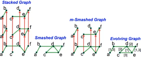
Figure 2:Various representations of temporal graphlets for the TGS in Fig. 1. A stacked graph is constructed by drawing directed edges in the direction of time between successive temporal graphlets in a TGS; a smashed graph is a “collapsed” version of the stacked graph. Alter-natively, it is union of the graphlets. Both smashed and m-smashed graphs are “lossy” representations.

3.

PRELIMINARIES

3.1

Temporal Graph

Assume slotted time starting at time0. Slott > 0starts just after timet−1and ends at timet. For0≤T1≤T2, aTemporal

Graphlet Sequence(TGS) is defined as

T GS(T1, T2) ={G(t) = (V(t), E(t))}, T1≤t≤T2

This model attempts to capture its space-time trajectory (see Figure 1). EachG(t)is referred to as atemporal graphlet, agraphlet, or asnapshot. Alternate notations that we use, depending on the em-phasis, includeG(T1, T2),G[1, T](shifting the frame of reference

maintains properties),G[T](reference shifting is implied). Atemporal graph, calledT-graph, is a single-graph represen-tation of the TGS. Such represenrepresen-tations include thestacked graph (StG), thesmashed graph (SmG)and its generalization them-smashed graph (m-SmG), and theevolving graphas shown in Figure 2. For-mally,

DEFINITION 1. Given a TGSG[1, T], thestacked graph (StG)

of G[1, T] isStG = (VS, ES), where VS = ∪tV(t), ES =

∪tE(t)∪ECwhereEC=∪t,i(ui(t), ui(t+ 1)).

DEFINITION 2. Given a TGSG[1, T], thesmashed graph (SmG)

ofG[1, T]isSmG= (VM, EM), where each sequence ofu(t), u(t+

1), . . .is replaced by a single vertexu∈VM, andEM =∪tE(t)

with endpoints of edges mapped to the replaced vertices inVM.

DEFINITION 3. Given a TGSG[1, T], them-smashed graph (m-SmG)ofG[1, T]ism-SmG= (VM, EM), where the

smash-ing operation is not performed on the entireG[1, T]but on each of

G[1, m], G[m+ 1,2m], G[2m+ 1,3m], . . .instead.

We note that the "evolving graph” representation proposed in [7] which labels edges with the times at which they are active is equiv-alent to the stacked graph1but an evolving graph is not a traditional graph. Hence reducing to an evolving graph does not allow us to easily leverage existing algorithms or code.

3.2

Temporal Coloring

Temporal coloring (T-coloring) is the process/task of coloring a given temporal graph in a conflict free manner. Specifically, it is a vertex coloring problem with constraintdistance-1anddistance-2

1

And deleting the labels yields a smashed graph.

on a time varying graph such that these constraints are satisfied for every snapshot in theT-graph. Thedistance-1constraint means that every pair of adjacent nodes must receive different colors; the

distance-2constraint means that every pair of nodes with shortest distance less than or equal to2must receive different colors.

DEFINITION 4. Given a coloring constraint, aT-Coloring is a labeling functionC: [1, T]×V →Nof the vertices of a temporal graphG[1, T]such thatC(t, v)satisfies the coloring constraint for eacht∈[1, T]and2v∈V.

For example, aT-Coloring with thedist-2constraint is a labeling functionC:T×V →Nsuch that for anyt∈[1, T]andu, v∈V, ifdist(u, v)≤2, thenC(t, u)6=C(t, v).

InT-Coloring, we count the total number of colors used (de-noted byC) and the total number of times any vertex changes its color between graphlets (denoted byA). The total number of col-orsCis the maximum label used if the positive integers1,2, . . .

are the labels. Formally,

DEFINITION 5. Given a T-graphG[T1, T2], and a coloring

al-gorithm, graphlet Gi has its color set C(Gi) = {ci(vj)|vj ∈

V(G)}, ci∈Z+. Then the total number of color used isC =

max(ci(vj)), and the total number of times a color is changed is

A=

T2−1

X

i=T1

X

vj∈V(G)

ci(vj)6=ci+1(vj).

As mentioned in section 1, practical applications require min-imizing both the number of colors and the number of color re-assignments. Accordingly, we define a simple and natural cost function to evaluate the quality of a T-coloring.

DEFINITION 6. Thecostof aT-coloringXis given byCOST(X) =C(X) +α·A(X)whereα≥0is a user defined parameter, and

CandAare, respectively, the total number of colors used and the total number of re-assignments as defined above.

3.3

Greedy Static Coloring

Our temporal coloring algorithms use as a key component a col-oring of a graphlet. Colcol-oring a graph is NP-hard to even approx-imate within a constant factor for both distance-1 and distance-2 constraints [13, 26]. While our temporal coloring algorithms are agnostic to the particular choice of static coloring method, includ-ing exponential-time optimal, we use a greedy heuristic from [18] called UxDMA with Progressive Minimum Neighbor First (we call it simply PMNF) ordering. Our implementation of PMNF has a running time ofO(|V||E|). However, one may replace PMNF with any other algorithm without impact on fundamental contributions, and therefore we shall refer to the procedurestatic-coloring.

4.

BASELINE ALGORITHMS: SNAP AND

SMASH

The set of possibleT-coloring algorithms for the cost function

COST =C+αAcan be thought of as lying along a spectrum that balances the number of colors and number of re-assignments in different ways. We begin by describing and theoretically analyzing two simple and naive algorithms at the two ends of that spectrum. These algorithms are oblivious to the value ofα.

2

(4)

Algorithm SNAP colors every snapshotG[Ti]in the stacked graph

independently and afresh using a static coloring algorithm (e.g. PMNF discussed in section 3.3). In this section, SNAP “ignores” the coloring ofG[Ti−1]when it colorsG[Ti]. In later sections, we

show that a greedy version of SNAP could do better if, for example, it considers the vertices in the same order for all theTgraphlets.

Algorithm 1SNAP for T-Coloring

Input:T-GraphG[1, T], constraint∈{dist-1,dist-2}

Output: Color assignment of each graphlet:Color[1, T]

1: fori from 1 to Tdo

2: Color(i)=static-color(Gi, constraint)

3: end for

4: returnColor[1, T]

Algorithm SMASH colors the smashed graph (refer definition in section 3.1) and the colors stay the same for allT graphlets. In other words, we simply run the static coloring algorithm on

SmG(G)with, say,Ccolors. We observe thatA= 0andCost=

C. The main drawback of SMASH is that it smashes all theT

graphs, thus creating a graph whose chromatic number is too high. In later sections, we show that partial smashing could help reduce the chromatic numbers at the cost of having some color changes.

Algorithm 2SMASH for T-Coloring

Output: Color assignment:Color(same for all graphlets) 1: G=SmG(G[1, t]))

2: Color=static-color(G, constraint) 3: returnColor

For the simple implementation of PMNF that was sufficient for our experiments, the worst-case running time of SNAP isO(|V|3

T) and that of SMASH isO(|V|3₊_|_V_|2_T₎

. Thus, SMASH is superior in running time.

We now consider the relative theoretical performance of SMASH and SNAP with respect toα, first with a worst-case viewpoint, then for Erdos-Renyi random graphs. First, we introduce some addi-tional notation fordist-2coloring. LetG2denote thedist-2graphlet that results from adding an edge between any two nodes inGthat are within two hops away from each other. Also, letSmG(G2₎

de-note the smasheddist-2T-Graph=SM ASH(G21, . . . , G2T)and

SmG2(G)denote thedist-2smashed T-Graph= (SM ASH(G1,

..., GT))2. It is easy to show that SmG(G2) is a subgraph of

SmG2(G).

4.1

Properties of SNAP and SMASH

For clarity, consider an optimal static coloring usage for SMASH and SNAP. However, the following discussion is valid for any “rea-sonable” greedy alternatives as well.

For the rest of this section, we assume thedist-1constraint, un-less otherwise specified. The next two propositions give thresholds for which one strategy outperforms the other for any T-graph.

PROPOSITION 1. Whenα > 1, SMASH is always better than SNAP.

PROOF. Suppose we color the T-graph with a SNAP algorithm

X, then we could define a new coloring: each time a vertex changes its color betweenGi andGi+1, we color this vertex with a new

unique color inG1...Gi+1. At the end of this process, the

col-oring is a legal T-colcol-oring of the smashed graph that usesC =

C(X) +A(X) colors. Obviously,C ≥ C(SM ASH), there-foreC(SM ASH) ≤C(X) +A(X) < C(X) +αA(X)since

α >1.

We remark that the above proposition is not true for dist-2 T-coloring on the original T-graph(G1, G2, . . . , GT). However, it is

true if both SMASH and SNAP were operating in dist-1 mode on the T-graph(G2

1, . . . , G2T).

PROPOSITION 2. Whenα = 0, SNAP is at least as good as SMASH.

PROOF. Whenα = 0, there is no penalty for changing colors and so cost of SNAP is the chromatic number under the optimal static coloring assumption. The chromatic number is monotonic in the sense that its value for a graphGis at least its value for any sub-graph ofG. Therefore,C(Gi) ≤ C(G). Thus, the cost of

SNAP is no larger than the cost of SMASH.

Given the above, a natural question is: in the intermediate values of0< α <1, which one is better? In particular, asαis increased above0, at what point does SNAP start to be worse than SMASH? We show that for an arbitrary sequence of graphlets there is no such threshold. However, for random graphlets such a threshold exists.

For the next two propositions we assume a “reasonable” imple-mentation of SNAP that does not try hard to avoid changes but also does not try to generate too many changes.

PROPOSITION 3. For anyα < 1, there exists a T-graph for which SNAP is better than SMASH.

PROOF. Letn = 3and call the verticesA, B, C. The edges

E ={(A, B),(A, C)}exist inG1whileE ={(A, B),(B, C)}

forG2, . . . , GT. The cost of SMASH is3since SMASH colors

the smashed graph with3colors. A “reasonable” SNAP uses only 2colors and changes the color ofConce for a total cost less than 3.

Note, that any greedy SNAP would use at most2colors and at most3changes. For an “adversarial” implementation of SNAP, the above proposition holds forα <1/3.

PROPOSITION 4. For anyα > 0, there exists a T-graph for which SMASH is better than SNAP.

PROOF. Letn= 4and call the verticesA, B, C, D. The edges

E={(A, B),(C, D)}exist inG1. A greedy or an optimal SNAP

will colorG1with2colors. Without loss of generality, assume that

AandCare colored with the color1. ThenE={(A, B),(A, C),(C, D)}

forG2, . . . , GT. A greedy or an optimal SNAP will colorG2, . . . , GT

with2colors but will have to change the color of at least2vertices. SMASH on the other hand will color the smashed graph with2 col-ors in a way that is good forG1as well. Sinceα >0, the cost of

SNAP is larger than the cost of SMASH for this T-graph.

Note that in the above example SNAP is paying the cost of not taking into account the future state of graphlets that SMASH is naturally able to do. Also note thatG2 is defined based on the

particular implementation of SNAP.

4.2

Analysis of T-coloring in Random T-graphs

In this section, we study properties of T-coloring in the simplest model of random T-graphs – each graphlet is an independently gen-erated graph obeying the Erdos-Renyi random graph modelER(n, p), in which, each of the possible n₂

edges exists with an independent probabilityp. We study the scaling of the number of colors neces-sary to color such graphs under bothdist-1anddist-2constraints as a function ofnandp.

(5)

4.2.1

Erdos-Renyi graphlets: dist-1 constraints

THEOREM5 (BOLLOBAS[3]). Letχg denote the chromatic

number under the greedy coloring algorithm,Gn,pis anER(n, p)

graph. Thenχg(Gn,p) = _logn 1 1−p

n, almost surely for any greedy

algorithm and any vertex ordering.

LEMMA 1. CSM ASH = χg(Gn,p0) = T ∗ n

log 1 1−p

n, where

p0= 1−(1−p)T.

PROOF. The smashed graph isER(n, p0)wherep0= 1−(1− p)T_{. Applying Bollobas’s theorem, we have:}_C

SM ASH =χg(Gn,p0) = n

log 1 1−p0 n

= n

log 1 1−(1−(1−p)T)

n=T∗ n

log 1 1−p

n. The last equality

is true sincelogxT n= (1/T) log_xn.

LEMMA 2. LetA0denote the expected number of color changes

between two consecutiveER(n, p)graphlets. ThenCOSTSN AP =

CSN AP+αASN AP = _logn₁ 1−p

n+α(T−1)A0.

PROOF. We rely on the assumption thatTis fixed whilentends to infinity, therefore, because of the concentration property in Bol-labas’ theorem mentioned above,CSN AP = max{C1, . . . , CT}=

n

log 1 1−p

n.

The next corollary follows from the above two lemmas.

COROLLARY 6. LetC0=_log n

1 1−p

n. Then with high

probabil-ity SNAP outperforms SMASH iffα < C0 A0.

We do not know how to boundA0 accurately. Obviouslynis

an upper bound onA0. Moreover, our simulations show thatA0is

almost surelyclose ton. Applying this upper bound to the above corollary, we have the following theorem.

THEOREM 7. For random Erdos-Renyi T-graphs, SNAP out-performs SMASH w.h.p. ifα≤ 1

log 1 1−pn

.

We conjecture thatA0is close tonand hence the above theorem

could be modified to be an “iff" theorem.

4.2.2

Erdos-Renyi graphlets: dist-2 constraints

We now show how Bollobas’ theorem mentioned in Section 4.2.1 could be applied underdist-2constraints as well. Some of the proofs have been omitted due to paucity of space. First, we give some basic results ondist-2coloring of single random graphlets and subsequently apply them to T-graphs.

LEMMA 3. The expected number of two hop neighbors in an Erdos-Renyi random graphG(n, p)isE[Nu(2)] = (n−1)((1−

p)(1−(1−p2)n−2)).

LEMMA 4. The expected number of nodes inside the two hop neighborhood in an Erdos-Renyi random graphG(n, p)is(n−

1) 1−(1−p)(1−p2₎n−2

.

PROOF. This follows from Lemma 3, the fact thatE[Nu(1)] =

(n−1)p, and linearity of expectation.

THEOREM 8. Letχ(2)g (Gn,p)be the number of colors used by

the greedy coloring algorithm under dist-2 constraints. Then,χ(2)g (Gn,p)∼

χg(Gn,p) +_logn(n−2) 1 1−p2

n.

Figure 3: dist-1anddist-2coloring of Erdos-Renyi GraphsG(n = 100, p). Forp∈[0.05,0.2],G(n= 100, p)is neither fragmented, nor is it a complete graph.

PROOF. We use Lemma 4 to create an equivalent (approximate) Erdos-Renyi graphG(n, q), whereq= 1−(1−p)(1−p2)n−2 denotes the probability of forming an edge between any nodeuand a nodewithinthe two hop neighborhood ofuinG(n, p). Then, we plug in this value ofqinto Theorem 5 to get the above estimate of

χ(2)g (Gn,p).

Even though Bollobas’ theorem is an asymptotic result, i.e., valid for large enoughnfor a certain fixed value ofp, Figure 3 shows that the performance of a greedy T-coloring algorithm can be rea-sonably predicted by applying Bollobas’ theorem under not only

dist-1constraints but alsodist-2constraints for a range ofpvalues for which the underlying graph has a non-trivial multi-hop struc-ture.

Assuming each graphlet in T-graph(G1, . . . , GT)is an

Erdos-Renyi graphG = ER(n, p), we haveG2 = ER(n, q), where from the proof of Theorem 8 we could say approximatelyq= 1−

(1−p)(1−p2₎n−2

.

OBSERVATION 9. For a T-graphG[1, T],SmG(G) =ER(n, pT),

where pT = 1−(1−p)T; SmG(G2) = ER(n, qT1), where

qT1 = 1−(1−q) T

; andSmG2(G) =ER(n, q2T), whereq

2

T =

1−(1−pT)(1−p2T)n −2

.

OBSERVATION 10. Underdist-2T-coloring, let

COST(SN AP) = C0+α(T−1)A0. ThenC0 =χg(G2) = n

log 1 1−q

nandA0≤n.

LEMMA 5. In dist-2 model, for any T-Graph (G1, . . . , GT),

χg(SmG(G2))≤χg(SmG2(G)).

THEOREM 11. In random Erdos-Renyi T-graphs, SNAP out-performs SMASH w.h.p. under dist-2 constraints ifα≤ 1 log 1

(1−p)(1−p2 )n−2n

.

PROOF. We find a lower bound forCOST(SM ASH).

COST(SM ASH) = χg(SmG2(G))≥χg(SmG(G2))

= n

log 1 1−q1_T

n =T χg(G

2

) =T C0

SinceA0 ≤n, so whenα= _log 1

1 (1−p)(1−p2 )n−2

n, from Obs. 10

we haveα= 1 log 1

1−q

n ≤ C0

A0;COST(SN AP) =C0+α(T−

(6)

5.

ENHANCED ALGORITHMS

In this section, we describe algorithms that seek to improve on the simple baseline algorithms from Section 4. We present two broad classes of algorithms. The first class seeks to enhance SNAP by reducing the number of re-assignments, for instance, by avoid-ing the independency in the coloravoid-ing of successive graphlets. The second class seeks to enhance SMASH by alleviating the creation of very dense graphs that necessitates the high number of colors. In the following subsections we describe two algorithms for the first class and four for the second class.

5.1

Progressive SNAP (P-SNAP)

The main drawback of the PMNF greedy algorithm in coloring the graphlets is that the coloring might need many re-assignments even if there is little change between two consecutive graphlets. The idea behind the Progressive SNAP algorithm is to useone

labeling (the PMNF forG1) for all the graphlets. Then, if the

graphlets evolve slowly, the coloring will remain the same for most of the vertices in the graph. Our experimental results, detailed later, bear this out.

Algorithm 3Progressive SNAP for T-Coloring

Output: Color assignment for each graphlet:Color[1, T]

1: label=PMNF-labeling(G1)

3: Color(i)=static-color(Gi,label,constraint)

4: end for

5.2

Incremental (INC)

The Progressive SNAP algorithm ignores the actual changes be-tween consecutive graphlets with the hope that a fixed global label-ing would reduce the number of reassignments. The INC algorithm on the other hand adopts a very local approach. It tries to minimize the number of reassignments for each graphlet. That is, it re-colors only the vertices whose coloring from the previous graphlet is ille-gal. In particular, when an edge appears between two vertices and causes a color conflict, INC changes the color of each of the two vertices using the “first-fit" natural strategy. When an edge disap-pears, INC does not try to reduce the number of colors because it tries to avoid reassignments. This process repeats itself until all conflicts due to new edges are resolved.

The INC algorithm is roughly similar to the one in [15], with some key differences – we do not re-color on edge deletions, we don’t attempt to perform “maintenance" of the coloring (both to avoid re-assignments). Also, in the [15] model, fixed position nodes appear and disappear, while in our model edges appear and disappear as a result of node mobility.

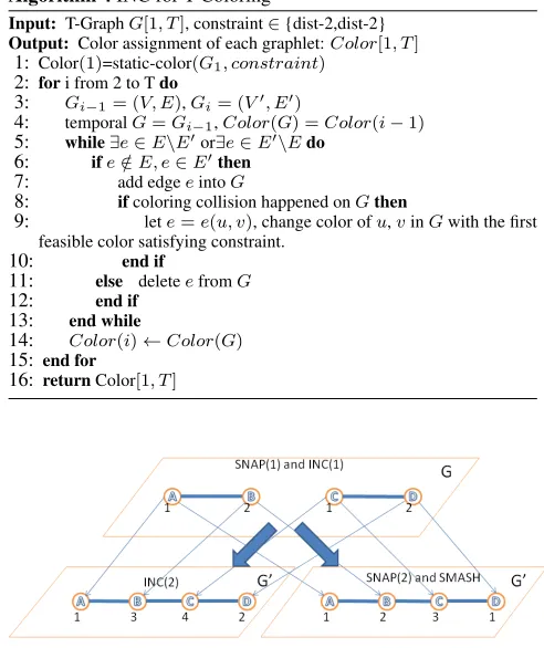
Intuitively, this strategy seems to be the best given our cost func-tion. However, as is the case with the greedy approach, there are cases in which both baseline algorithms SNAP and SMASH out-perform INC. An example is illustrated in Figure 4.

5.3

m-SMASH

Unlike the previous two strategies which were based on SNAP, the m-SMASH strategy is based on SMASH. The main drawback of SMASH is that the smashed graph might require too many colors and having no reassignments would not help reducing the COST. m-SMASH proposes a simple solution – it smashes intervals ofm

consecutive graphlets and generates a dynamic graph with about

T /mgraphlets. These graphlets are then colored using a SNAP strategy.

Algorithm 4INC for T-Coloring

Input: T-GraphG[1, T], constraint∈{dist-2,dist-2}

Output: Color assignment of each graphlet:Color[1, T]

1: Color(1)=static-color(G1, constraint)

3: Gi−1= (V, E),Gi= (V0, E0)

4: temporalG=Gi−1,Color(G) =Color(i−1)

5: while∃e∈E\E0or∃e∈E0\Edo

6: ife /∈E, e∈E0_then 7: add edgeeintoG

8: ifcoloring collision happened onGthen

9: lete=e(u, v), change color ofu,vinGwith the first feasible color satisfying constraint.

10: end if

11: else deleteefromG

12: end if

13: end while

14: Color(i)←Color(G)

15: end for

Figure 4:An example of when INC does worse than SNAP & SMASH: SNAP and INC will both color the first graphlet(2K2)in color

se-quence(1,2,1,2). While INC will color the second graphlet(L4)in

color sequence(1,3,4,2), SNAP will color this graphlet in color se-quence(1,2,3,1). SMASH will color the smashed graph of these two graphlet in color sequence(1,2,3,1)too. Thus, in this case, INC uses4 colors and number of color changes is2; SNAP uses3colors and num-ber of color changes is1; SMASH only uses3colors. Therefore, for any

α≥0, the cost of INC is strictly greater than both INC and SMASH.

Algorithm 5m-SMASH

Input: T-GraphG[1, T], integerm(< T), constraint∈{dist-1,dist-2}

Output: color assignment of each graphlet:Color[1, T]

2: ifm\iori=Tthen

3: Coloring each graphlet in G[i− bi

mc+ 1, i]with static-color(SmG(G[i− bi

mc+ 1, i]), constraint)

4: end if

5: end for

6: returnColor[1,T]

OBSERVATION 12. For T-coloring a T-graphG[1, T], m-SMASH is equivalent to SNAP whenm= 1and to SMASH whenm=T.

Recall that for smallα → 0, SNAP outperforms SMASH al-most everywhere; and forα → 1, SMASH outperforms SNAP almost surely. For a givenα, a natural problem is to find the best value form such that m-SMASH would outperform both SNAP and SMASH. Denote such a value bym(α).

OBSERVATION 13. Under dist-1 constraints,m(0) = 1, and

(7)

5.4

Big-Change-SMASH (BC-SMASH)

The m-SMASHing algorithm is easy to implement. However, it ignores actual changes between consecutive graphlets. The BC-SMASH examines the T-graph snapshot by snapshot, and then de-termines the intervals to be smashed. Intuitively, when graphlets evolve slowly, the coloring set for each graphlets will be similar to each other, and similar to the coloring set for the smashed graph of these graphlets. Based on this intuition, BC-SMASH looks for two adjacent graphlets that are very different. The steps are shown in Algorithm 6.

Algorithm 6Big-Change-SMASH

Input:T-GraphG[1, T], integerK(≤T), constraint∈{dist-2, dist-2}

1: fori from 1 to T-1do

2: di←the difference betweenGiandGi+1

3: end for

4: Sortingd1,· · ·, dT−1, letdp1,· · ·, dpK−1be the largest K-1 ones (assuming0 =p0< p1< ... < pK−1< pK =T)

5: fori from 0 to K-1do

6: Color each graphlet in G[pi + 1, pi+1] with

static-color(SmG(pi+ 1, pi+1), constraint)

7: end for

8: returnColor[1,T]

5.5

Accumulated-Error-SMASH

The main drawback of the Big-Change-SMASH algorithm is that the sum of many small numbers could be very large. In many cases, the BC-SMASH algorithm smashes large intervals in which consecutive graphlets are similar but the smashed graph represent-ing this interval requires too many colors. The Accumulated-Error-SMASH algorithm (Algorithm 7) is a more sophisticated approach that findsKintervals each with about the same number of changes between its boundary graphlets. The total complexity of Algorithm 7 isO(Kn2₎

.

Algorithm 7Accumulated-Error-SMASH

Input:T-GraphG[1, T], integerK(≤T), constraint∈{dist-1 dist-2}

1: fori from 1 to T-1do

2: di←the difference betweenGiandGi+1

3: end for

4: By dynamic programming find partitioning points pi, such that

0 = p0 < p1 < p2, ... < pK = T for objective function

minp1,...,pK(maxi(

Ppi

j=pi−1+1dj))

5: fori from 0 to K-1do

6: Color each graphlet in G[pi + 1, pi+1] with

static-color(SmG(G[pi+ 1, pi+1]), constraint)

7: end for

8: returnColor[1,T]

As was the case with m-SMASH, the two extreme cases for both Algorithms 6 and 7 are SNAP (K=T−1) and SMASH (K= 1), respectively. A open question is to find the bestKfor a givenα.

5.6

Adaptive Hybrid

SNAP, P-SNAP, and INC, although simple, do not perform well across all ranges ofαor parameters of the RGG-RWP model (de-tails in Section 6). Moreover, they do not utilize any knowledge of the parameters of the T-graph evolution (whether given or learnt). In this section, we present a hybrid approach that utilizes the avail-able model information and switches between two algorithms, de-pending on the current level of network dynamics.

Our proposed hybrid algorithm (Algorithm 8) essentially sets an edge-change threshold for deciding whether to switch between T-coloring (pure) strategies P-SNAP and INC. For small values of

α, the value ofCOSTis dominated byC, hence P-SNAP (which attempts to lowerC) is the suitable coloring scheme; on the con-trary, for higher values ofα,COSTis dominated byA, hence INC (which attempts to avoid recoloring a vertex, unless essential) is the suitable T-coloring scheme.

Consider consecutive graphletsGandG0which are both RGGs and let∆(G, G0)be the symmetric difference between the edge sets of two graphs, i.e.,(E\E0)∪(E0\E). By means of simu-lation, we found that due to the spatial nature of the RGG, the r.v.

|∆(G, G0)|is quite concentrated around its expected value, which can be shown to be bounded as follows (see Appx A):E[|∆(G, G0)|]<

n(n−1) 2

2πrs D2 = ∆

∗ .

Rather than using a fixed threshold across all values ofα, Algo-rithm 8 uses an adaptive threshold function, which is a decreasing function ofα, and is denoted byθ(∆, T, α). The rationale behind the choice ofθ(∆, T, α)is as follows: if the expected number of edge changes between consecutive graphlets is∆and each edge change typically triggers no more than one recoloring, the con-tribution of the expected “recoloring" cost to the totalCOST is

A(∆, T, α) = ∆T α. For fixed∆, T, the multiplier terme−A(∆,T ,α)

varies from1to0asαincreases above0. This achieves the adap-tive switching behavior described earlier (see Sec. 6 for perfor-mance evaluation).

Algorithm 8Adaptive Hybrid

Input: (Any two consecutive graphletsG, G0 _∈ _G_[1_{, T}_]_{; valid coloring} of graphletG; RGG-RWP model parametersr, s, D, n, constraint∈ {dist-1, dist-2}

Output: color assignment of graphletG0

1: ∆∗=n(n−1)πrs_D2

2: θ(∆, T , α) = 2e−∆T α_∆

3: if|∆(G, G0₎_|_{> θ}_(∆∗_{, T , α}₎_then

4: Color(G0) = Algorithm INC(G, G0,constraint) 5: else

6: Color(G0) = Algorithm P-SNAP(G0, P M N F −labeling(G), constraint)

7: end if

8: returnColor(G0₎

6.

EXPERIMENTAL ANALYSIS

In this section, we evaluate conflict-free channel assignment (over a period of time) in a MANET modeled as temporal graph color-ing. We evaluate by simulation the performance of the various tem-poral coloring schemes described in sections 4 and 5 on a random MANET whose nodes follow the random waypoint mobility model (RWP). The parameters used in the simulation study are given in the table below. Note that all possible combinations of parameters in the table were not simulated.

Parameter and Description Range

n(Number of nodes) 50,100

D(Side of square area) 1000

s(Node speed) 5,10,15,20

r(Transmission range) [25,200]

T(Time window of evaluation) 100,200

α(Significance of reassignment) [0.0001,1]

K(Budget for smashing algorithms) 10,20

m(Number of graphlets compressed form-SMASH) ∼[T K]

(8)

Figure 5:For most values ofαP-SNAP outperforms SNAP, especially at lower speeds and higher range.

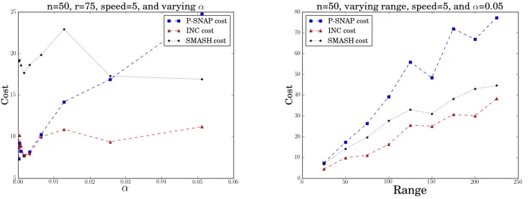
Figure 6:INC outperforms both P-SNAP and SMASH. The relative performance of P-SNAP and SMASH depends upon the parameters.

We focus on “pivot" or “crossover values", that is, when the rel-ative performance (cost)of two or more algorithms reverse them-selves. Recall that cost isC+αAwhereCis the total #colors,A

total #re-assignments, andαis a user-defined parameter.

We note that SNAP, P-SNAP, INC and hybrid strictly require only one snapshot at a time whereas SMASH,m-SMASH, BC-SMASH, AE-SMASH require the entire T-graph. In order to com-pare all algorithms with the lowest common denominator of re-quirement, we assume all algorithms receive the full T-graph.

In all experiments below, we generate a T-graph based on the random geometric graph (RGG) with random waypoint mobility model (RWP). In theRGG(n;D;r)model, nnodes are placed uniformly randomly in aD×D square, and two nodes have an edge between them iff they are within a transmission ranger. In theRW P(n;D;s)mobility model, each node picks a destination uniformly randomly in the square and moves to it at a constant given speeds, then picks another destination, and so on. There is no “pause time" at the destination. A T-graph is generated as follows. At each time slott, graphletG(t)is the RGG based on vertex positions at timet, and we store each graph letG(t)as a stacked graph for T-coloring.

In the generation of RGG and RWP, we use generic “units" – one may assign any (the same) transformation from “units" to ac-tual metrics (e.g. 1 unit could be 10 meters). All experiments below are done using an RGG withn= 50andD = 1000. The speed, range and the cost biasαare varied differently for each of the ex-periments. All of the colorings done use thedist-2constraint which

represents broadcast scheduling for TDMA and is the most appli-cable vertex coloring constraint in practice. Each point in the plot represents an average over 50 random T-graph samples for all al-gorithms except Adaptive Hybrid for which we used 20 samples to accommodate its higher running time.

We first compare SNAP and P-SNAP. For this set of experiments, the radiusr= 75. Figure 5 shows the percentage improvement of P-SNAP over SNAP as a function ofαfor varying RWP speeds and ranges. We observe that for all but very small values of α

P-SNAP outperforms SNAP. As discussed earlier in section 5, for dynamism at the rates studied, two consecutive graphlets are nearly the same, and using the same ordering obviously results in better performance. At very lowα, the cost is essentially the number of colors used. PMNF labeling is very effective in reducing the colors used, and since SNAP always uses PMNF while P-SNAP uses it only once at the beginning, whenαis very small, SNAP uses less colors than P-SNAP.

We also observe that P-SNAP outperforms SNAP to a greater extent at lowersand higherr. Lower speeds result in similar con-secutive graphlets, thus increasing P-SNAP’s advantage of “sticky" labeling. At higher ranges, the graphlets are more connected and have a higher chromatic number. The higher number of colors re-sults in a larger gap between re-assignments in SNAP and P-SNAP. Given that P-SNAP outperforms SNAP for most of the parame-ter space of inparame-terest, we use P-SNAP going forward, and compare it with SMASH and INC. For this set of experiments,r= 75and

(9)

algo-Figure 7:SMASH, m-SMASH, Big-Change-SMASH exhibit a "pivot" or "crossover" point, at approximatelyα=0.05

rithm as a function ofαandr. INC outperforms both SMASH and P-SNAP. Thus, although we showed in section 5 that there are instances where INC incurs greater cost than both SMASH and P-SNAP, it appears that this is not evident in practice, at least in the RGG-RWP model.

However, there is no clear "winner" between SMASH and P-SNAP. There is a value ofα, approximately0.05, below which P-SNAP is better, and above which SMASH is better. At higher

α, re-assignments are more costly and SMASH does not re-assign. Further, as the plot on the right in Figure 6 shows, forα= 0.05, the gap between SMASH and P-SNAP widens with increasing range. A denser graph is more suitable for SMASH since then the differ-ence between a single graphlet and a smashed graph narrows.

We now compare the different kinds of smashing algorithms, namely m-SMASH, Big-Change-SMASH (BC-SMASH), and reg-ular (full) SMASH. For this set of experiments, Figures 7(a,b) show the results as a function ofαfor budgetsK = 10andK = 20, for different values ofr. We observe an interesting phenomenon around a “pivot" value ofα: whenαis less than the pivot value, the cost is in the order B-C-SMASH<m-SMASH<SMASH, and whenαis greater than this pivot value the cost is reversed as SMASH<m-SMASH<BC-SMASH. It is particularly interesting that the crossovers between the three algorithms occurat the same point, and for different combinations of range andK(we have ob-served this in other combinations not shown here due to lack of space). We observe that the pivot point moves to the right with decreasingK.

Figure 7(c) shows the cost versusratα= 0.05. A crossover can be seen between BC-SMASH and SMASH (with m-SMASH outperforming both).

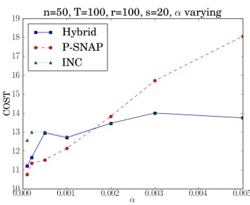
Finally, we evaluate the performance of the adaptive hybrid al-gorithm (Alal-gorithm 8) that switches between two online schemes P-SNAP and INC based on the current network dynamics and the value ofα. Figure 8 illustrates that Algorithm 8 adaptively switches from P-SNAP (at lowα) to INC (at higherα). Note that the thresh-old functionθ(·)given in Algorithm 8 is only illustrative, and other more complex functions can indeed be used instead.

Our experiments provide a way by which a user can select the right algorithm based on the kind of network, i.e„ the cost bias between colors and re-assignments, and range, among other things.

7.

CONCLUDING REMARKS

We have considered the problem of channel assignment in mo-bile or otherwise dynamic networks as a graph coloring problem. We have presented a model with two novel components: a tem-poral graphand an associated temporal coloring model; and a

Figure 8:Hybrid online algorithm switches between P-SNAP and INC asαis varied

cost modelC+αAthat allows a user-selectable tradeoff between number of colors (channels), and their changes over time. Using this model, we have presented a suite of algorithms ranging from simple ones such as SNAP, P-SNAP and SMASH, to more so-phisticated ones such as INC,m-SMASH, Big-Change-SMASH, Accumulated-Error-SMASH, and an adaptive hybrid algorithm.

For SNAP and SMASH, we have derived bounds for when one outperforms the other, for arbitrary graphs as well as Erdos-Renyi random graphs. For all algorithms, we have presented experimental results with typically used placement and mobility models. Our study shows that there exist crossover or pivotαpoints between pairs or triplets of algorithms, withα = 0.05figuring as a kind of “magic number". Our work, with suitable adaptations, can be applied to time-, frequency- or code-based medium access in a real-life multi hop wireless network, and guide a designer to select the right algorithm for her preferredα.

Many exciting avenues for future work exist. These include fur-ther extending the theoretical bounds for distance-2 coloring and for other algorithms, especially budget-based ones, improving the performance of the online algorithms, extending to a physical prop-agation model and distributed implementations.

8.

REFERENCES

[1] F. S. Al-Anzi, Y. N. Sotskov, A. Allahverdi, and G. V. Andreev. Using mixed graph coloring to minimize total completion time in job shop scheduling.Applied

(10)

[2] N. Alon, A. Bar-Noy, N. Linial, and D. Peleg. On the complexity of radio communication. InProc. of the 21st ACM symposium on Theory of computing, pages 274–285. ACM, 1989.

[3] B. Bollobás. The chromatic number of random graphs.

Combinatorica, 8(1):49–55, 1988.

[4] B. Bollobás.Random graphs, volume 73. Cambridge university press, 2001.

[5] A. Ephremides and T. Truong. Scheduling broadcasts in multihop radio networks.Communications, IEEE Transactions on, 38(4):456–460, 1990.

[6] P. Erd˝os and A. Rényi. On the evolution of random graphs.

Magyar Tud. Akad. Mat. Kutató Int. Közl, 5:17–61, 1960. [7] A. Ferreira. Building a reference combinatorial model for

MANETs.Network, IEEE, 18(5):24–29, 2004.

[8] P. Gupta and P. R. Kumar. The capacity of wireless networks.

IEEE Transactions on Information Theory, 46:388–404, 2000.

[9] W. Hale. Frequency assignment: Theory and applications.

Proceedings of the IEEE, 68(12):1497–1514, 1980.

[10] L. Hu. Distributed code assignments for CDMA packet radio networks. InProc. IEEE INFOCOM ’91, pages 1500–1509, 1991.

[11] S. Khuri, W. Moh, and F. Chung. Code assignments in CDMA networks: distributed algorithms and genetic algorithm heuristics. InProc. of the 6th IEEE Singapore International Conference on Networks, volume 98, pages 91–105, 1998.

[12] V. Kostakos. Temporal graphs.Physica A: Statistical Mechanics and its Applications, 388(6):1007 – 1023, 2009. [13] E. Lloyd and S. Ramanathan. On the complexity of

distance-2 coloring. InComputing and Information, 1992. Proceedings. ICCI ’92., Fourth International Conference on, pages 71 –74, may 1992.

[14] E. Lloyd and S. Ramanathan. Efficient distributed algorithms for channel assignment in multihop radio networks.Journal of High Speed Networks, 2(4):405–428, 1993.

[15] X. Ma and E. Lloyd. An Incremental Algorithm for Broadcast Scheduling in Packet Radio Networks. In

MILCOM, volume 1, pages 205–210, 1998.

[16] C. McDiarmid and T. Muller. On the chromatic number of random geometric graphs. Technical report, Oxford University, 2011. http://arxiv.org/abs/1101.6065. [17] A. Panconesi and A. Srinivasan. Improved distributed

algorithms for coloring and network decomposition problems. InProc. of the 24th ACM symposium on Theory of computing, pages 581–592. ACM, 1992.

[18] S. Ramanathan. A unified framework and algorithm for channel assignment in wireless networks.Wireless Networks, 5(2):81–94, 1999.

[19] S. Ramanathan and E. Lloyd. Scheduling algorithms for multihop radio networks.IEEE/ACM Transactions on Networking (TON), 1(2):166–177, 1993.

[20] R. Ramaswami and K. Parhi. Distributed scheduling of broadcasts in a radio network. InProc. IEEE INFOCOM ’89, pages 497–504. IEEE, 1989.

[21] J. Redi and R. Ramanathan. The DARPA WNaN network architecture. InMILITARY COMMUNICATIONS

CONFERENCE, 2011 - MILCOM 2011, pages 2258 –2263, Nov. 2011.

[22] S. Scellato, I. Leontiadis, C. Mascolo, P. Basu, and M. Zafer. Evaluating Temporal Robustness of Mobile Networks.IEEE Transactions on Mobile Computing, 12(1):105–117, 2013. [23] Y. Shi, Y. T. Hou, J. Liu, and S. Kompella. Bridging the gap

between protocol and physical models for wireless networks.

IEEE Trans. Mob. Comput., 12(7):1404–1416, 2013. [24] J. Wang and B. Prabhala. Periodicity Based Next Place

Prediction.the Procedings of Mobile Data Challenge by Nokia Workshop at the Tenth International Conference on Pervasive Computing, June 2012.

[25] J. Whitbeck, M. Dias de Amorim, V. Conan, and J.-L. Guillaume. Temporal reachability graphs. InProc. Mobicom ’12, pages 377–388, 2012.

[26] A. Wigderson. Improving the Performance Guarantee for Approximate Graph Coloring.J. ACM, vol. 30, No. 4, pages 729–735, Oct 1983.

[27] H. Wu, F. Yang, K. Tan, J. Chen, Q. Zhang, and Z. Zhang. Distributed channel assignment and routing in multiradio multichannel multihop wireless networks.Selected Areas in Communications, IEEE Journal on, 24(11):1972–1983, 2006.

APPENDIX

A.

COMPUTING THRESHOLD

∆∗

FOR

HY-BRID ONLINE T-COLORING

We calculate the expected number of edge-changes between two RGG-RWP graphletsG, G0. The model parameters are: area (D× D), number of nodes (n), connectivity radius (r), and speed (s). We assume thatGis a uniformly distributed RGG, and the future direc-tion of each node is chosen randomly. Consider an edge(A, B)in

G. Due to RWP mobility,A→A0andB →B0(change of loca-tions inG0). Define eventsY = 1(A,B)∈GandZ = 1(A0_,B0₎_∈_G0.

Then, we have,E[∆(G, G0)] =n(n₂−1){Pr(Z|Y¯) Pr( ¯Y)+Pr( ¯Z|Y) Pr(Y)}. By assumingD >> r, we havePr(Y) = πr2

D2 andPr( ¯Y) =

1−πr2

D2. For fixed parametersr, s, define the following function:

f(x) = Pr(|AB| = x,|AA0| = s,|BB0| = s,|A0B0| < r). After geometric probability calculations (omitted due to paucity of

space), it can be shown thatf(x) = 1

π π

R

0 1

R

0

Pr(|AB|=x, B0 =

B+ 2aseiθ_,_|_A0

B0|< r)dθda. Forx≤r−2s, f(x) = 1. For

x≥r−2s, letθ∗(x) = arccos((2s)2₂+_sxx2−r2). So1> f(x)>

1−1 2(1−

θ∗(x)

π )(1− r−x

2s ). Therefore, we have:

Pr( ¯Z|Y) = 1−

Z r

0

2x

r2(1−f(x))dx <

s(3r−2s) 3r2

Pr(Z|Y¯) = 1−

Z D

r

2πx

D2₋_πr2(1−f(x))dx <

πs(3r+ 2s) 3(D2₋_πr2₎

Therefore, it follows thatE[∆(G, G0)]<n(n₂−1)2_Dπrs2 .

OBSERVATION 14. It is obvious that if|AB| < r−2s, then

|A0B0|< r; and if|AB|> r+ 2s, then|A0B0|> r, therefore, a naive upper bound is given by

Pr((A, B)changing)<π(r+ 2s)

2₋_π₍_r₋₂_s₎2

D2 =

8πrs D2