Artisan Studio ParaSolver Tutorials

(1)

Atlanta, GA 30332, USA Voice: +1-404-592-6897 Web: www.InterCAX.com E-mail: [email protected]

Artisan Studio ParaSolver™

7.2 R1

Tutorials

Table of Contents

1 Introduction and review ... 3

1.1 Introduction ... 3

1.2 Short Review of SysML ... 4

Short Review of Solving Equations ... 6

2 SysML Parametrics Tutorial - Addition ... 7

2.1 Objective ... 7

What the User Will Learn ... 7

2.2 Step-by-Step Tutorial ... 7

Step I Create Model ... 7

Step II Create Structural Model ... 9

Step III. Create Constraints ... 10

Step IV Create Parametrics Model ... 10

Step V Create an Instance ... 12

Step VI Solve the Instance ... 14

3 SysML Parametrics Tutorial - Satellite ... 16

3.1 Objective ... 16

Step I Create Model ... 16

Step III Create Constraints ... 18

4 SysML Parametrics Tutorial - LittleEye ... 26

4.1 Objective ... 26

Step I Create Project ... 27

(2)

5 SysML Parametrics Tutorial - CommNetwork ... 34

5.1 Objective ... 34

Step V Create Parametrics Model(s) ... 37

6. SysML Parametrics Tutorial - Orbital ... 42

6.1 Objective ... 42

System Requirements ... 43

6.2 Step-by Step Tutorial ... 43

7. SysML Parametrics Tutorial - HomeHeating ... 54

7.2 Step-by Step Tutorial ... 55

8. SysML Parametrics Tutorial – LittleEye Trade Study ... 61

8.2 Step-by-Step Tutorial ... 61

Step VII Set-up a Trade Study ... 61

(3)

1

I

N

1 IN

TRODUCTION AND REVIEW

TRODUCTION

AND

REVIEW

1.1 Introduction

The primary purposes of SysML up to this point have been Documentation, precise specification of system design, and Communication, sharing the design among multiple parties. Adding parametric execution to SysML enables additional purposes,

• Consistency, enforcing internal relationships to insure a coherent, self-consistent data set; • Simulation, evaluating the performance, cost and other parameters of the system design; • Verification, integrating checks of system properties against requirements;

• Operations, moving the system model from development to ongoing operational use.

Our general approach for creating SysML model with parametrics follows the pattern

I. Create Model

II. Create Structural Model III. Create Constraints IV. Create Parametric Model V. Create an Instance VI. Solve the Instance

Steps I and II are equivalent to those already performed by SysML users and it is generally straightforward to add parametrics to existing models. Step III, Constraints, has the user define the generic mathematical relationships to be used. Step IV “wires up” the connections between numerical attributes in the structural model and the constraint equations, using one or more SysML Parametric diagrams. In Step V, the user must create a specific example of the model, populating some of the attributes in the model with real numbers and identifying others as unknowns to be calculated in Step VI. This outline is not offered as a general methodology for building parametric models, so much as a helpful outline for organizing the detailed instructions.

Before the user can reproduce these tutorials, the user must install and configure • Artisan Studio 7.0.20 with SysML profile

• ParaSolver, the InterCAX SysML Parametrics plug-in for Artisan Studio • Mathematica 7 (Wolfram Research) and/or OpenModelica 1.5.0

Several features of the tutorial models are specific to Artisan Studio 7.0.20 and ParaSolver 0.54 and may not work correctly with earlier versions. Contact Artisan or InterCAX for further information.

The fifth and sixth tutorials use two additional tools: • Microsoft Excel

• MATLAB (The MathWorks, Inc.) with the Simulink toolkit

In each case, refer to the installation instructions in the appropriate user guide. It is also necessary to modify ParaSolver so that it points to the copy of Mathematica. We assume that Artisan Studio, ParaSolver, OpenModelica, MATLAB and Excel (if required) are all installed on the user’s local machine. Mathematica may be local or accessed through a web services interface.

(4)

but with the Artisan Studio SysML profile, as well. In the later tutorials, we will hide more of the procedural detail and describe several labor-saving short-cuts, as we model more complex and realistic systems. Occasional Notes discuss the “why” of certain procedures.

The second tutorial, Satellite, models the weight and power budgets of a satellite system, introducing concepts of hierarchy, requirements and multiple constraints. The third tutorial, LittleEye, models the operational capability of an unmanned aerial vehicle, introducing object-oriented programming in model design and non-arithmetic functions. The seventh tutorial extends this model to trade studies. The fourth tutorial, CommNetwork, introduces the use of simple elements to build up and simulate more complex networks.

The fifth and sixth tutorials provide an introduction to special features for interfacing to Excel and MATLAB. The Orbital tutorial shows how Excel may be used to load initial values into a model for space mission planning and to record parametric simulation results. The HomeHeating tutorial demonstrates how external functions programmed in MATLAB can be integrated into the parametric simulation. Both these tutorials require Mathematica as the core solver to execute; OpenModelica does not support solving MATLAB and Mathematica functions.

As with many subjects, the best way to learn SysML Parametrics is by doing. The author recommends building the models described in the first four tutorials, comparing your results with the figures in the text and exploring variations. There are generally multiple ways to implement any model and, in a few cases, alternate procedures are described. The author would appreciate user feedback on errors and unclear descriptions in this document ([email protected]).

1.2 Short Review of SysML

SysML is a powerful and wide-reaching language for modeling systems. In this section, we will review a few aspects of SysML of special importance to parametrics, to help make sense of the detailed instructions in the tutorials for new users with limited SysML experience. This is not intended as a broad introduction or primer on SysML.

SysML supports three major classes of diagrams, which are ways at the looking at the system model:

• Structure diagrams, which describe what the system is composed of. Parametrics is part of structure and these diagrams are our principal focus in the tutorials.

• Behavior diagrams, which describe what the system does. We will not deal with any behavior diagrams, which do not support parametrics at this time.

• Requirements diagrams, which describe the design and performance objectives the system must meet. We introduce a requirements diagram in the tutorial Satellite, to show how parametrics can help build requirements checking into a system model. Within structure diagrams, there are three important types. These are illustrated in Figure 1.1.

• Block definition diagrams (BDD), which describe the organization of the structure, the hierarchy of system, subsystems, and all the elements that make up the system. In Figure 1.1, the Body, Engine, and Wheels are elements that belong to the object Automobile, the ownership relationships shown in black. Our tutorials usually begin by creating a BDD.

• Internal block diagrams (IBD), which describe qualitative flows between elements. In Figure 1.1, gasoline flows from a tank in the Body to the Engine, as shown in red. In the tutorial CommNetwork, we use an IBD to keep track of message traffic channels

(5)

• Parametric diagrams (PAR), which describe quantitative relationships between

properties of the elements. In Figure 1.1, mileage, which is a property of Automobile, is a function of the drag of the Body, the efficiency of the Engine, and so forth in green. Creating and executing parametric diagrams is the primary focus of these tutorials.

Figure 1.1 Structure diagram relationships

Finally, we need to clarify three types of objects within the system: blocks, part properties, and instances. Examples are illustrated in Figure 1.2.

• Blocks represent a generic object, like the Wheel in Figure 1.2a. A block may have value properties which describe it, like model number or radius, but these properties typically do not contain specific values.

• Part properties represent usages of a block; i.e. a block as part of some larger system. In Figure 1.2b, Front Wheel and Back Wheel are two separate roles that Wheel plays as part of Motorcycle.

• Instances represent a specific example of a generic object, like WhiteWallRadial in Figure 1.2c. The value properties have specific values, which may be fixed or calculated from other system values. ParaSolver executes parametric calculations for specific instances of system models.

(6)

Short Review of Solving Equations

ParaSolver’s primary function is to solve the often-complex network of parametric equations within the system model, so it is valuable to review a few concepts that will come up in the tutorials.

Causality is the organization of known and unknown variables in the equations. ParaSolver requires the assignment of a causality state to each variable, which can be done manually by the user or semi-automatically by the ParaSolver program. The allowable causality states are

• Given – a parameter with a known value provided by the user before the ParaSolver calculation.

• Target – a parameter with an initially unknown value that the user specifically wishes to calculate. Each ParaSolver calculation requires at least one target variable.

• Undefined – a parameter with an initially unknown value, that may be calculated in the process of solving for the target.

• Ancillary – an undefined parameter after its value has been calculated by ParaSolver. It can’t be assigned before solution.

As an example, consider the two equation network

a + b = c c + d = e

Our objective is to calculate e, which is assigned target causality. If we know beforehand that a

= 3, b = 2, and d = 5, these parameters would be assigned given causality. The remaining

parameter, c, could be assigned undefined causality. When we solve for e, the causality of c

changes from undefined to ancillary. It is also possible to assign both c and e to target causality,

but multiplying targets unnecessarily may slow down solving for larger equation sets.

Assigning causality requires consideration of overconstraint/underconstraint. Underconstraint occurs when insufficient variables are assigned values and given causality to calculate the

targets. For example, in the equations above, if we set a = 3 and d = 5, there are an infinite number of solutions for e and the equation set is underconstrained. Alternately, if we assigned a = 3, b = 2, d = 5, and e = 6, the system is overconstrained and there are zero possible solutions for c. In general, Mathematica, the solver engine for ParaSolver, will alert the user when overconstraint/underconstraint occurs, but some analysis by the user might be required to determine the correct number of knowns for complex equation sets.

(7)

2

S

Y

2 SY

S

ML P

ML

P

ARAMETRICS

T

UTORIAL

- A

-

A

DDITION

2.1 Objective

Create a SysML project with three elements. Each element has one attribute. The attribute of the third element is the sum of the first two attributes. Create an instance of this model and solve for the third attribute parametrically.

Figure 2.1 Outline of Objective What the User Will Learn

• Creating the basic elements of SysML models in Artisan Studio: blocks, properties, constraints, etc.

• Building a SysML parametrics model and diagram

• Creating a instance of the model with input and output parameters • Opening and using the ParaSolver browser window

• Exporting a parametrics model to Mathematica

2.2 Step-by-Step Tutorial

Step I Create Model

1. Open Artisan Studio 2. Create a new model

a. On Artisan Studio menu bar, select File→New Model,

b. In the New Model window (Figure 2.2), check ParaSolver under Systems Engineering. Several other boxes will be checked automatically,

c. Set Name = Addition and use default repository.

d. Click OK. The Creating Model window displays the process, which may take several minutes.

3. Create a package within the project

a. RC (Right-click) on Addition model in Packages pane (Figure 2.3) b. Select New→Package (Figure 2.4).

(8)

Figure 2.2 New Model window

Figure 2.3 Packages pane Figure 2.4 Creating a new package

(9)

Step II Create Structural Model

4. Create elements in model

a. RC (Right-click) the Addition package in the Packages pane i. Select New→SysML Blocks→Block

ii. Enter Name = Alpha in blank text box in Packages pane or in Properties window

b. RC Addition

i. Select New→SysML Blocks→Block ii. Name = Beta

c. RC Addition

i. Select New→SysML Blocks→Block ii. Name = Gamma

d. RC Alpha in Packages pane

i. Select New→Block Property (Value)

ii. In the Type Selector window which appears (Figure 2.6), choose ValueTypes from the Types pull-down box at the bottom

iii. Expand the All Value Types entry in the Existing Types window by clicking on the plus sign beside it

iv. Select Real and click OK.

v. Enter Name = a in blank text box in Packages pane or in Properties window.

e. RC Beta

i. Select New→Block Property (Value) 1. Type = Real

2. Name = b f. RC Gamma

i. Select New→Block Property (Value) 1. Type = Real

2. Name = c Figure 2.6 Type Selector

window

5. Create a block definition diagram, a graphical view of the entire system a. RC the Addition package in Packages pane

b. Select New→Diagram→Block Definition Diagram i. Name = AdditionBDD

c. Drag Alpha, Beta, and Gamma from Packages window to BDD i. To rearrange position, drag block.

ii. To resize block, click on block and use cursors at edges and corners iii. To display block properties,

1. RC on a block in the diagram,

(10)

6. Create relationships between elements of the model. Alpha and Beta will be considered as parts of Gamma, so we will create Part Properties of type Alpha and Beta within Gamma.

a. Select Directed Composition connector from top toolbar (solid black diamond with line to right)

Figure 2.7 Block Definition Diagram

i. Click on Gamma in the Block Definition Diagram

ii. Click on Alpha

b. Repeat steps a 1 and 2 for Beta (Figure 2.7)

c. This procedure causes blocks Alpha and Beta to be mirrored as Part Properties inside Gamma, initially with the names BlockProperty1 and

BlockProperty2. Rename these Part Properties as alp and bet, respectively, in the Packages or Properties windows.

d. The block definition diagram should now look similar to Figure 2.7.

Step III. Create Constraints

7. Create a constraint block, which contains a mathematical relationship that the model will use.

a. RC the Addition package in the Packages window i. Select New→SysML Blocks→Constraint Block

1. Name = AdditionEqn b. RC AdditionEqn

i. Select New→Constraint Parameter

1. Select ValueType as real (see Step 4.d.ii) and Name = a. ii. Repeat for constraint parameters b and c

c. Click on Constraint1 under Add

i. Under Properties window, General tab, rename constraint as sum. ii. Under Properties window, Full Text tab, enter c = a + b

Step IV Create Parametrics Model

8. Create a SysML Parametric diagram to define and display the relationships inside Gamma

a. RC Gamma in Packages window b. Select New→Parametric Diagram

i. Set Name = Gamma

(11)

i. A yellow constraint block will appear inside Gamma (in the Packages tree and in the parametric diagram) as a Constraint Property of the type AdditionEqn. Assign it a unique name, add1.

ii. To display the constraint, RC on add1 and Select Toggle Compartments→Constraints

iii. To display the constraint parameters, RC on add1 and Populate→Constraint Parameters.

iv. Resize and arrange constraint parameters as shown in Figure 2.8.

d. Drag the Part Properties alp:Alpha and bet:Beta, and the Value Property c from under Gamma in the Packages pane to the parametric diagram

i. To display the value property a within Part Property alp, RC on alp:Alpha and Populate→PAR-Block Properties (Value).

ii. Repeat for b in bet:Beta.

iii. Reposition and resize parts and part properties for alp, bet and c as shown in Figure 2.8.

Note: In general, Toggle Compartment, Populate, and View Options provide control in displaying or hiding properties and other elements inside blocks.

e. Create connections between value properties of blocks, the structural elements of the model, and constraint parameters, the expressions of mathematical relationships these elements obey.

i. Click the Connector icon in the top toolbar. ii. Click c.

iii. Click the constraint parameter c in add1. iv. A black line will connect c and c.

v. Repeat this process for b in bet:Beta and b in add1, and for a in alp:Alpha and a in add1.

vi. The final parametric diagram should be similar to Figure 2.8.

(12)

f. Create the CXS Heading.

i. RC on block Gamma in the Packages pane.

ii. Select Tools→ParaSolver→Util→Create CXS_heading.

iii. Click F5, or select View→Refresh All from the Studio menu, to see the CXS Heading as an element in the Packages pane under the Package Addition.

Note: The CXS Heading contains the schema of the parametric network that ParaSolver will solve. Clicking on Gamma identifies it as the root block, the highest level block contained within the network.

Step V Create an Instance

9. Create an instance. An instance is an example of the model with specific values assigned to the given parameters and which can be solved for the unknown(s).

a. RC the Addition package in the Packages pane. i. Create New→Package, Name = Instance01 b. RC Instance01

i. Create New →Instance Model→Object Diagram, Name = Instance01 ii. Create New →Instance Model→Instance,

1. Set Name = gamma01

2. Drag gamma01 into the Object Diagram

3. To shorten the name of instance, RC the block and select View Options. Check only Show Name and Show Slots.

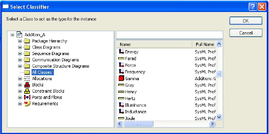
4. In Properties window for gamma01, Type tab, click Select button. 5. In Select Classifier window (see Figure 2.9), select All Classes in

tree on left, then select gamma from list on right and click OK. iii. Repeat step ii for instance alpha01 of type Alpha and beta01 of type

(13)

Figure 2.9 Instance Specification

c. Create links from gamma01 to alpha01 and beta01 i. Click on Link icon on top toolbar

ii. Click on gamma01 iii. Click on alpha01

iv. A black line with the label alp will link the two elements v. Repeat this process for gamma01 and beta01.

d. Activate the slots for known and unknown parameters in the parametric calculations.

i. Click on alpha01

1. In the Properties window, Slot Values tab, click under the Text Value column header in the row for a.

2. Enter 20 <Enter> as the value for a.

3. a = 20 should appear in the instance block alpha01. It may be necessary to resize the box to see it.

ii. Click on beta01 and repeat for the value 10. iii. Click on gamma01.

1. In the Properties window, Slot Values tab, click under the Text Value column header in the row for c.

2. Enter <Enter> as the value for c.

3. c should appear in the instance block gamma01.

e. Create the CXI Heading.

i. RC on the Instance01 package in the Packages pane. ii. Select Tools→ParaSolver→Util→Create CXI_heading.

(14)

f. The Instance diagram should appear similar to Figure 2.10. Note the elements in the final model tree in the Packages pane.

Figure 2.10 Instance Diagram and final model tree

Step VI Solve the Instance

10. Run the parametric solver

a. RC Instance01 in the Packages pane.

b. Select Tools→ParaSolver→Browse. Click Expand and the browser should appear similar to Figure 2.11a. Alternatively, individual elements can be expanded or collapsed by clicking on the small selector switch icons on the left edge.

c. In order to solve, at least one element must be assigned target causality. To

change the causality of C, click on the causality for that parameter and a drop-down menu will show the available options, as in Figure 2.11b. Select target.

d. Figure 2.11c shows the Browser ready for solution, with the Solve button active. e. Click Solve. Figure 2.11.d shows the Browser after solution.

f. Click Update to SysML to upload the results of the calculation into the instance in the SysML model.

(15)

Figure 2.11a ParaSolver Browser window, on initial opening and expansion

Figure 2.11b ParaSolver Browser window, showing causality selection

Figure 2.11c ParaSolver Browser window, after causality selection

Figure 2.11d ParaSolver Browser window, after solution

(16)

3

S

Y

3 SY

S

ML P

ML

P

ARAMETRICS

T

UTORIAL

- S

-

S

ATELLITE

3.1 Objective

Create a SysML project comprising a satellite system composed of four subsystems: Propulsion, Instrumentation, Control and PowerSystem. Each subsystem has a weight and there is a total weight budget for the satellite of 10,000 kilograms. The Propulsion, Instrumentation, and Control subsystems each draw electrical power from the PowerSystem, which can supply a maximum of 10 megawatts. Given the weights of all four subsystems and the power requirements of three, calculate the total weight and power demand for the system and compare against requirements.

Figure 3.1 Outline of Objective

What the User Will Learn

• Apply SysML parametrics to a realistic system with subsystems • Working with multiple constraints

• Working with requirements • Working with ValueTypes

• Changing causality – reversing the direction of calculation

3.2 Step-by-Step Tutorial

Step I Create Model

1. Create new SysML/ParaSolver model, Name = SimpleSat 2. Create a package within the model, Name = Satellite

Step II Create Structural Model

a. Set-up units to be used in model

(17)

ii. RC ValueTypes and select New→SysML Blocks→ValueType, Name = Kg (kilograms will be the unit for weight in our model)

iii. RC ValueTypes and select New→SysML Blocks→ValueType, Name = KW (kilowatts will be the unit for power in our model)

Note – ValueTypes, Units, and Dimensions

We frequently want to apply units to a value property, for example, electrical power in our model will be expressed in kilowatts. We can use the Type property to make this assignment. Assigning valuetypes to properties makes the model more exact and helps identify mismatches when block properties and constraint parameters are linked in parametric diagrams. The full description of the relationship between ValueTypes, Units and Dimensions is described in the Artisan Studio User Guide.

4. RC on Satellite, create New→SysML Blocks →Block, Name = SatelliteSystem a. In SatelliteSystem, create three new value properties

i. Name = Weight, Type = Kg

ii. Name = Weight_MOS, Type = Real iii. Name = Power_MOS, Type = Real

5. RC on Satellite, create four new blocks with value properties, as follows a. Name = Propulsion, with two value properties

i. Name = Wpro, Type = Kilogram ii. Name = Ppro, Type = Kilowatt

b. Name = Instrumentation, with two value properties i. Name = Wins, Type = Kilogram

ii. Name = Pins, Type = Kilowatt c. Name = Control, with two value properties

i. Name = Wcon, Type = Kilogram ii. Name = Pcon, Type = Kilowatt

d. Name = PowerSystem, with two value properties i. Name = Wpsy, Type = Kilogram

ii. Name = Power, Type = Kilowatt

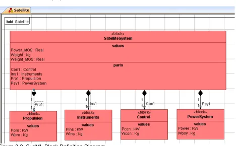
6. RC on Satellite,

i. Create New→Diagram→Block Definition Diagram, Name = Satellite ii. RC on diagram Satellite and select Populate→Blocks. The five blocks

created in Steps 4 and 5 will appear in the diagram.

Note – Using the Populate command avoids having to drag each of the blocks into the diagram separately. We will use this command later to create the parametrics diagram as well.

iii. Draw Direct Composition connectors (solid black diamond) from

(18)

iv. The Satellite block definition diagram should appear similar to Figure 3.2. Use the Toggle Compartments command to display part and value

properties inside each block.

Figure 3.2 SysML Block Definition Diagram

Step III Create Constraints

7. Inside the Package pane create two constraint blocks, which contain mathematical relationships that the model will use for weight and power calculation

a. RC Satellite, select New→SysML Blocks→Constraint Block, Name = WeightBalance

i. Under WeightBalance, click Constraint1, Name = weightdemand, Full Text w = w1 + w2 + w3 + w4

ii. RC WeightBalance, select Tools→ParaSolver→Util→Infer Parameters iii. Five constraint parameters, w, w1, …, will be created. Reset the value

type for each to Kg in the Properties window, Data Type tab. Note – The Infer Parameters utility in ParaSolver can expedite building constraint blocks. However, all parameters are set by default to Real value type, which may require retyping, like here.

b. RC Satellite, select New→SysML Blocks→Constraint Block, Name = PowerBalance

i. Under PowerBalance, click Constraint1, Name = powerdemand, Full Text p = p1 + p2 + p3

(19)

iii. Five constraint parameters, p, p1, …, will be created. Reset the value type for each to KW in the Properties window, Data Type tab.

8. Create a Requirements diagram to show the specifications for the Satellite system. The purpose of a Requirements diagram is to make clear the requirements the system must meet and how these requirements tie to specific values of the model. For our purpose, we can pair each Requirement with a Constraint Block that mirrors it, making it easy to automatically verify the constraint when ParaSolver is executed.

a. RC on Satellite, create New →Package, Name = SatelliteSpecification b. RC on SatelliteSpecification, create New→ Diagram→Requirement Diagram,

Name = SatelliteSpecification c. Create two new requirement blocks

i. RC on the SatelliteSpecification package, create New→ SysML Requirements →Requirement, Name = WeightReqt

1. In Properties window, Requirement tab, enter the ID number, 1.0.1, under Tag Value for id#

2. In Properties window, Text tab, with Description in the top pull-down menu, enter the requirements text = Total system weight must be less than 10,000 kilograms.

ii. Create a second requirement block, Name = PowerReqt, id = 2.0.1, text = Total system power use must be less than 10,000 kilowatts iii. Drag both requirements blocks into the requirements diagram.

d. Create two new constraint blocks that verify the requirements

i. RC on the SatelliteSpecification package, create New→SysML Blocks→Constraint Block, Name = WeightMOS (where MOS is margin of safety)

1. Under WeightMOS, create two constraint parameters, mos with value type Real and actual with value type Kg

2. Rename constraint as wtmos, with Full Text mos = (10000 - actual)/10000.

3. This constraint calculates the margin of safety in total system weight, positive if actual is below 10,000 (kg) and negative if above.

ii. Create a second constraint block, Name = PowerMOS , with a constraint, Name = pwmos, Full Text = mos = (10000 - actual)/10000

iii. Drag both constraint blocks into the requirements diagram. e. In the requirements diagram, create a Satisfy relationship between each

constraint block and the requirement it verifies.

i. Click on the Satisfy icon on the top toolbar (s above arrow). ii. Click on WeightMOS.

iii. Click on WeightReqt.

iv. A Satisfy dependency arrow is created linking the objects. This identifies the relationship, but has no effect on parametric calculations at this time.

(20)

f. The final requirements diagram should be similar to Figure 3.3.

Figure 3.3 SysML Requirements Diagram

Step IV Create Parametrics Model

9. Create a SysML Parametric diagram to define and display the relationships inside SatelliteSystem

a. RC SatelliteSystem

b. Create New→Parametric Diagram, Name = PAR_SatelliteSystem c. RC inside PAR_SatelliteSystem and select Populate→Block Properties

(Part). The four subsystems will appear. For each, select Populate→PAR_Block Properties (Value).

d. RC inside PAR_SatelliteSystem and select Populate→Block Properties (Value). Three value properties appear, but Power_MOS and Weight_MOS should be selected and deleted from the diagram (do not choose Delete from model). They will be connected in a second parametric diagram.

(21)

f. Draw connectors between value properties and constraint parameters as shown in Figure 3.4.

Figure 3.4 SysML Parametrics Diagram

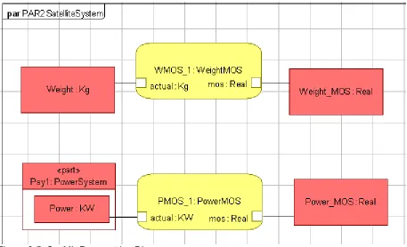
10. Create a second SysML Parametric diagram to define and display the calculation of the requirements verification relationships inside SatelliteSpecfication

a. RC SatelliteSystem

b. Create New→Parametric Diagram, Name = PAR2_SatelliteSystem c. Drag Psy1 into PAR2_SatelliteSystem. Select Populate→PAR_Block

Properties (Value). Delete Wpsy.

d. RC inside PAR2_SatelliteSystem and select Populate→Block Properties (Value). Three value properties appear, Weight, Power_MOS and Weight_MOS.

e. Drag the WeightMOS and PowerMOS constraint blocks from the

SatelliteSpecification package into the diagram and name the constraint properties created WMOS_1 and PMOS_1, respectively. Click on each, select Populate→Constraint Parameters, and rearrange and resize the constraint properties in the diagram as shown in Figure 3.5.

f. Draw connectors between value properties and constraint parameters as shown in Figure 3.5.

11. Create the CXS_heading and validate the model schema, a. RC on SatelliteSystem in the Packages pane and select

(22)

Figure 3.5 SysML Parametrics Diagram

Step V Create an Instance

11. Create an instance of the model.

a. RC the Satellite package in the Packages pane. i. Create New→Package, Name = Instance01 b. RC Instance01

i. Create New →Instance Model→Object Diagram, Name = Instance01 ii. Create New →Instance Model→Instance, Name = Sat01, Type =

SatelliteSystem

iii. Drag Sat01 to Instance Diagram

iv. Repeat steps ii and iii for instance Pro01 of type Propulsion, Ins01 of type Instrumentation, Con01 of type Control and Psy01 of type PowerSystem. c. Create links from Sat01 to Pro01, Ins01, Con01, and Psy01.

i. Click on Link icon on top toolbar ii. Click on Sat01

iii. Click on Pro01

iv. A black line with the label Pro1 (the part property name) will link the two elements

v. Repeat this process for the other subsystems.

d. Activate the slots for known and unknown parameters in the parametric calculations.

i. Click on Sat01

(23)

2. Hit <Enter> (or double-click) to set an empty value for the slot, which will be an unknown in this instance.

3. Repeat process for slots Power_MOS and Weight_MOS ii. Set values for the subsystem value properties

1. Wpro: Kg = 5000 2. Ppro: KW = 5000 3. Wins: Kg = 2000 4. Pins: KW = 2000 5. Wcon: Kg = 1500 6. Pcon: KW = 500 7. Wpsy: Kg = 2000 8. Power: KW (empty) e. Create the CXI Heading.

i. RC on the Instance01 package in the Packages pane. ii. Select Tools→ParaSolver→Util→Create CXI_heading. f. The Instance diagram should appear similar to Figure 3.6.

Figure 3.6 Satellite Instance_01 Diagram

Step VI Solve the Instance

12. Run the parametric solver

a. RC Instance01 in the Packages pane.

b. Select Tools→ParaSolver→Browse. Click Expand and the browser should appear similar to Figure 3.7a

c. Change Power_MOS and Weight_MOS to target causality, by clicking on the

(24)

Discussion – Causality

The Browser assigns a causality to each active parameter when it is opened; given for

parameters with assigned values and undefined for parameters with empty values. However, at

least one slot must be re-assigned target causality for ParaSolver to seek a solution. Typically,

these will be the final results, not intermediate results.

One parameter in each independent system of equations should be a target. For example, in this tutorial, if Weight_MOS is assigned as a target and Power_MOS as undefined, no value for Power_MOS will be calculated since that equation is independent from the weight calculation. However, assigning all unknowns as target may slow down solving, by initiating calculations not required for the desired result.

A fourth causality state, ancillary, is assigned after solution. This indicates parameters

solved for as intermediate results.

d. Figure 3.7a shows the Browser ready for solution, with the Solve button active. e. Click Solve. Figure 3.7b shows the Browser after solution.

Figure 3.7a ParaSolver Browser for Instance_01, before solution

Figure 3.7b ParaSolver Browser for Instance_01, after solution

Note – Causality

Mathematica is a non-causal solver, that is, it can solve many equations in any direction. The user can take advantage of this to use the same model to answer different kinds of questions. However, not all solvers are non-causal (e.g. Microsoft Excel formulas work in one direction only) and not all functions work in multiple directions (e.g. A = MINIMUM(B,C,D) cannot be solved exactly for D given A, B and C). Keeping track of causality can require some effort on the part of the modeler.

(25)

package become the unknown, we can use the same model to determine the maximum weight allowable for the instruments package (assuming, in this case, that the weight of the other subsystems is fixed.).

f. Change the causality of Weight_MOS to given and set the value to 0.

g. Change the causality of Wins to target. The browser should appear like Figure

3.8a.

h. Click Solve. The final browser is shown in Figure 3.8b.

Figure 3.8a ParaSolver Browser for

Instance_01, after change in causality, before solution

(26)

4

S

Y

4 SY

S

ML P

ML

P

ARAMETRICS

T

UTORIAL

- L

-

L

ITTLEEYE

ITTLE

E

YE

4.1 Objective

The third tutorial demonstrates the use of SysML to determine operational performance using a sequence of equations. The system is the LittleEye unmanned aerial vehicle (UAV) which is used to provide reconnaissance. The objective is to calculate how many miles of road can be scanned per 24 hours, which will be determined by the number and duty cycle of aircraft, the number and duty cycle of crews, and the availability of fuel.

The complexity of the model, with six elements, eight constraints and more than twenty parameters, makes it a good place to introduce “object-oriented” modeling techniques, which allow a complex model to be built from simple, independent and potentially reusable subsystems, tied together only at the highest levels

What the User Will Learn

• Applying an “object-oriented” approach to SysML parametrics

• Embedding constraints and parametric diagrams within multiple blocks in the model • Using standard functions, e.g. Minimum

• Using simulation to explore a model with “what-if scenarios”

(27)

Step I Create Project

1. Create new SysML project, Name = LittleEye 2. Create new Package, Name = LittleEye

Step II Create Structural Model

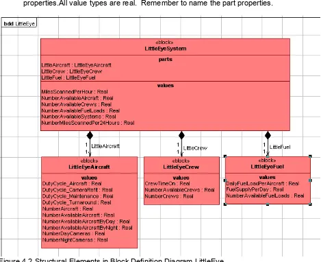
3. Using the procedures described in the previous tutorials, create the Block Definition Diagram as shown in Figure 4.2 containing the four blocks with value and part properties.All value types are real. Remember to name the part properties.

Figure 4.2 Structural Elements in Block Definition Diagram LittleEye

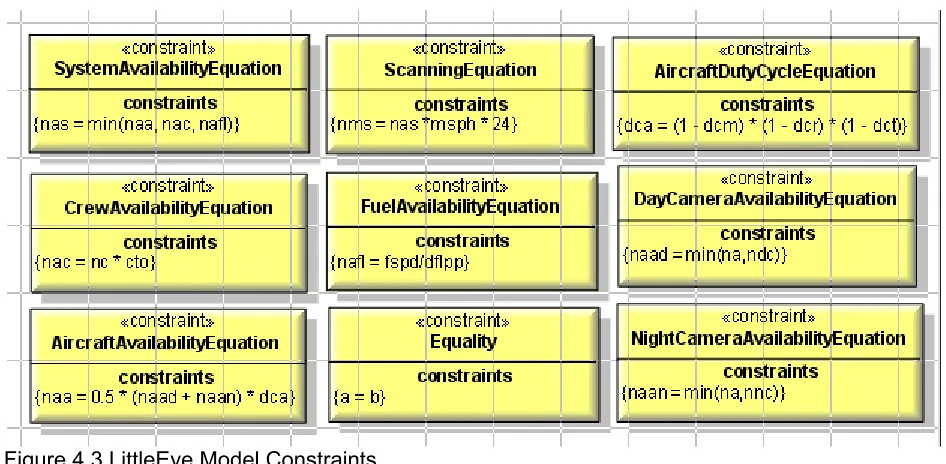
Step III Create Constraints

(28)

Figure 4.3 LittleEye Model Constraints Note – Object-Oriented Modeling

An important feature of object-oriented modeling is the modularity of important subsystems, which enhances collaboration and reusability. In this model, several parameters which link different blocks are mirrored, i.e. they appear in two different block and will be linked by equalities in a high level parametric diagram. For example, NumberAvailableAircraft appears as a value property in both the LittleEyeSystem and LittleEyeAircraft blocks. The internal relationships in each block can then be modified independently as long as the identity of these “boundary” parameters is constant.

If a constraint block is unique to a specific block, e.g. the CrewAvailabilityEquation to the LittleEyeCrew block, the modeler may let the block own the constraint block, not just the constraint property based on that constraint block. The “owner” of the block can more easily modify and re-use the block with this kind of organization. However, if the constraint block is used in multiple places within the model, this approach may cause problems.

Step IV Create Parametrics Model

5. Using an “object-oriented” programming approach, the four elements of Figure 4.2 will be converted into independent submodels containing internal constraints and

relationships

a. The submodel LittleEyeSystem will contain the six values listed in Figure 4.2 plus two constraints that connect them, the Scanning Equation and the System

Availability Equation at the top of Figure 4.3. See Figure 4.4.

i. In LittleEyeSystem, create a New→Parametric Diagram, Name = LittleEyeSystem

ii. Drag the six values inside LittleEyeSystem in the Packages pane onto the parametrics diagram (or use the Populate→Block Properties (Value) command).

iii. Create a new Constraint Property by dragging the Constraint Block ScanningEqn into the parametrics diagram, Name = SE. Use the

(29)

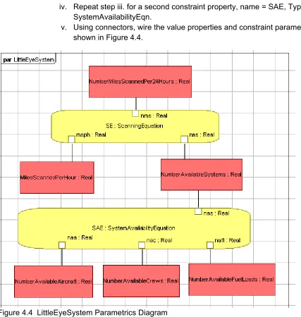
iv. Repeat step iii. for a second constraint property, name = SAE, Type = SystemAvailabilityEqn.

v. Using connectors, wire the value properties and constraint parameters as shown in Figure 4.4.

Figure 4.4 LittleEyeSystem Parametrics Diagram

b. Create submodels for the Aircraft, Crew, and Fuel blocks using the same

procedures, ending with the parametrics diagrams shown in Figures 4.5, 4.6 and 4.7.

Note – Equality Constraints

(30)

Figure 4.5 LittleEyeCrew Parametrics Diagram

Figure 4.6 LittleEyeFuel Parametrics Diagram

(31)

6. Create an overall parametrics diagram to connect the different submodels.

a. Create a second SysML Parametrics diagram inside LittleEyeSystem called LittleEyeSystem_2.

b. Drag the three part properties, LittleAircraft, LittleCrew and LittleFuel, into the parametrics diagram (or use the Populate→Block Properties (Part) command). c. Drag the three value properties, NumberAvailablePlanes,

NumberAvailableCrews and NumberAvailableFuelLoads into the parametric diagram (or use the Populate→Block Properties (Value) command).

d. Using the Populate→PAR_Block Properties (Value) command, display the internal structure of the three submodels as shown in Figure 4.8. Note that only the parameters necessary for wiring between the high-level model and the submodels are shown; all other parameters have been deleted from the diagram (but not from the model).

e. Create three constraint properties based on the Equality constraint block. f. Draw connectors between model properties as shown in Figure 4.8.

Figure 4.8 LittleEyeSystem_2 Parametric Diagram 7. Create the CXS_heading,

(32)

Step V Create an Instance

8. Create an instance of the model. The values for several of the givens are taken from Figure 4.1. Others, such as the Number of Planes, are user-set trial values, which will be varied during the solving operation.

a. Create a package called Instance01 inside the LittleEye package. b. Create an object diagram for the instance.

c. Create instances of System01, Aircraft01, Crew01 and Fuel01 with their respective Types.

d. Activate and assign values to known parameters using the Properties window, Slot Values tab.

i. It is necessary to use the notation 0.42 instead of .42 for decimal values or the ParaSolver browser will not be able to interpret the inputs

e. Link the Aircraft01, Fuel01 and Crew01 blocks to System01 block using the Link connector on the top toolbar.

f. Create a CXI_heading element inside Instance01 g. The final instance should appear similar to Figure 4.9.

Figure 4.9 An Instance of the LittleEye model

Step VI Solve the Instance

9. Solve the instance

a. Open the browser (ToolsÆParaSolverÆBrowse)

(33)

c. Click Solve.

d. The browser after solution should look like Figure 4.10. Note – Displaying Results

The Browser displays numbers truncated to a fixed maximum number of decimal places determined by the NumberOfDecimals parameter in the Artisan Software Tools\Artisan Real-time Studio\Exe\ParaSolver\conf\ParaSolver.ini.

Figure 4.10 Browser for Instance01 of LittleEye

Figure 4.11 Browser with an increase in number of crews

Note – Interpreting the Results

The target result, NumberMilesScannedPer24Hours, is 2,016 miles for this set of inputs. Deeper inspection shows that the number of available systems is 2.1, on average, and is limited by the number of available crews through the SystemAvailabilityEquation. The number of available aircraft, 2.4, and fuel loads, 5, are not the limiting factors in keeping UAVs in the air. Increasing the number of crews should increase the total number of miles scanned per 24 hours, as shown in Figure 4.11.

(34)

5

S

Y

5 SY

S

ML P

ML

P

ARAMETRICS

T

UTORIAL

- C

-

C

OMM

OMMNETWORK

N

ETWORK

5.1 Objective

The fourth tutorial uses SysML to simulate a simple communication network. The objective is to calculate the output of the network given the input and the loss in the individual channels between stations..

Figure 5.1 Outline of Network

The focus of this tutorial is working with limited number of standard elements to build up more complex structures. In this example, there are only two standard elements, stations (nodes) and channels. Each element contains constraint relations describing its behavior. An Internal Block Diagram is created to assist in completing the parametric diagrams correctly. Parametric constraints are also used at a higher level to define interactions between elements.

What the User Will Learn

• Building complex structures from multiple usages of simple structures • Using internal block diagrams

1. Create new SysML project and Package, Name = CommNetwork

Step II Create Structural Model

2. Create three blocks: Network, Node and Channel.

(35)

b. Node represents a station which can receive and transmit messages. It has two inputs, two outputs, and the ability to redistribute the message traffic depending on the capacity of the transmission channels. To build the node model, we will use flowports, value properties and parametric diagrams.

i. Each node has four flowports, two for receiving message traffic and two for transmitting (see Figure 5.2). To create a flowport

1. RC on Node, create New→FlowPort

2. In the Type Selector window, select No Type and OK (Figure 5.3). 3. In the Value Selector window, select in and OK (Figure 5.4). 4. Assign this flowport the name Rec1 in the Properties window or in

the Packages tree.

5. Repeat for other three flowports. Note that Direction is out for Trans1 and Trans2

Figure 5.2 Node with Ports Figure 5.3 Type Selector Figure 5.4 Value Selector

ii. The Node block has nine Value Properties, all Real. Six represent levels of message traffic at input and output, units unspecified: R1, R2, R, T1, T2, and T. Two represent the capacities of the upstream channels: C1 and C2. The final attribute, D, represents the redistribution factor in splitting outgoing message traffic between the Tr1 and Tr2 ports. c. Channel represents a two-way communication link between two stations. The

throughput of each line, the output signal divided by the input, is a function of the channel capacity C and the total signal traffic level. It has two inputs and two outputs, but may only use one I/O pair in a particular instance. To build the channel model, we will use flowports, value properties and parametric diagrams.

i. Each channel has four flowports, two for input message traffic (In1 and In2) and two for output (Out1 and Out2).

ii. The Channel block has six Value Properties, all Real. Five represent levels of message traffic at input and output, units unspecified: IT1, IT2, IT, 0T1, and 0T2. C represents the intrinsic capacity of the channel.

(36)

a. RC on CommNetwork package, create New→Diagram→Block Definition Diagram, Name = Network_BDD

i. Drag Network, Node and Channel blocks into the diagram (or use Populate→Blocks)

ii. Using the Composition connector from the top toolbar, connect as shown in Figure 5.5. Note that four connections are made from Network to Node, and the resulting four Part Properties are named Node1, Node2, Node3 and Node4. Similarly, five connections are made from Network to Channel, named as ChannelA thru ChannelE.

Figure 5.5 CommNetwork Block Definition Diagram

b. RC on Network block in Packages pane, create New→Internal Block Diagram, Name = Network IBD

i. RC in diagram and select Populate→Block Properties (Part) (or drag all nine part properties in Network (four node and five channels) into the diagram).

ii. Right-click on each block and select Populate→IBD FlowPorts. Arrange the parts and ports as shown in Figure 5.6.

(37)

Figure 5.6 CommNetwork Internal Block Diagram

Step III Create Constraints

4. Create the five constraint blocks required by the model: ErrorRate, Fraction, Product, Product1 and Sum. Usage of these constraint blocks are shown in the parametric diagrams in Figure 5.7 and 5.8, which show the constraints and constraint parameters for each.

Step V Create Parametrics Model(s)

5. Create a parametric model for CommNetwork. There are standard relationships internal to Node and Channel elements and there are equalities tying the Nodes and Channels together into a network.

a. Create a parametrics diagram within the Node block, Name = Node. This diagram, shown in Figure 5.7, contains five separate constraint properties, with the constraints shown, the nine internal value properties, and the connectors tying them together. Note that an Equality constraint property, eq1, is shown in a minimized format to save space. In this example, the objective of the equations to redistribute the incoming signal to the two outgoing channels, based on their relative capacities. No claim is made about the realism of this model.

b. To show the constraint within each constraint property, RC on the block and choose Toggle Compartment→Constraints. To hide the type (Real) of each constraint parameters, RC on each constraint parameter box, select View Options and uncheck Type. View Options can be applied to multiple selections.

6. Create a parametrics diagram within the Channel block, Name = Channel. This

(38)

Figure 5.7 Node parametric diagram

(39)

7. Create 4 parametric diagrams in the Network block connecting the channels and nodes through equalities as in Figure 5.09a-d. Use the internal block diagram in Figure 5.6 to keep track of which blocks and ports connect. In this example, we have chosen to divide the entire set of high level parametric relationships into four separate diagrams in order to keep each individual diagram simpler with fewer elements. This illustrates the

combined use of internal block diagrams for a high-level qualitative perspective and narrower parametric diagrams to make the actual quantitative connections. Note that the Equality constraint properties are shown in a minimized format to save space.

Figure 5.09a Node 1 parametric diagram

Figure 5.09b Node 2 parametric diagram

Figure 5.09c Node 4 parametric diagram

Figure 5.09d Node 3 parametric diagram

8. To create the CXS_heading,

a. RC on Network in the Packages pane and select Tools→ParaSolver→Util→Create CXS_heading

Step V Create an Instance

9. Create an instance of CommNetwork as in the previous tutorials. a. Create an Object Diagram, Name = Instance01

b. Create an instance of Network, Name = Net01

c. Create four instances of Node, Names = N1, N2, N3 and N4

(40)

e. Draw links from Net01 to the other nine instances, as shown in Figure 5.10. In each case, Artisan will offer a choice of the available part properties that instance could correspond to. Select Node1 as the part property for N1, Node2 for N2, and so forth.

f. Activate the value parameters in each instance block (Network contains no value properties), assigning a few given values as shown in Figure 5.10.

i. In N1, we set R1 = 10 and R2 = 0 to establish a starting level of traffic in the initial node.

ii. In N4, we set C1 = C2 = 0. Even though there are no further nodes or channel to consider, we need to provide non-empty values to prevent Mathematica from creating errors in trying to solve the signal distribution constraints that are part of all the Node models.

iii. An arbitrary capacity value of 5 for C is assigned for all the channels. iv. Channels A through D are assigned a secondary input value of 0 because

only one line is used in this network. The reverse line is used only in the crosschannel E.

Figure 5.10 Instance01 object diagram

10. Create a CXI heading in the Instance01 package by selecting Tools→ParaSolver→Util→Create CXI_heading.

Step VI Solve the Instance

(41)

a.

Set target causality for R in Node4. This is the total message traffic received at Node 4.

b. Click Solve. The final solution appears as in Figure 5.12. Note that Mathematica has not calculated a value for T, which is unnecessary to calculate the target parameter R.

Figure 5.11 Browser for Instance01 before solution

(42)

6

.

S

Y

S

M

L

P

A

R

A

M

E

T

R

I

C

S

T

U

T

O

R

I

A

L

-

O

R

B

I

T

A

L

6.1 Objective

Create a SysML project combining an orbital mechanics subsystem and a spacecraft subsystem. The orbital mechanics section is linked to a spreadsheet which calculated solar power levels and data transmission levels for ten sections in the spacecraft’s orbit around Mars, based on the geometry between the spacecraft, Mars, Earth and the Sun. See Figure 6.1. Note that the writer claims no expertise in this field.

The spacecraft subsystem is tied to a second spreadsheet which contains the power and data transmission requirements for the spacecraft by subsystems, three instrument packages, a transmitter, and a power system. Information from both spreadsheets is combined at the Mission level using parametric constraints solved by Mathematica and final results are written to a third spreadsheet.

What the User Will Learn

• Read and write between Microsoft Excel spreadsheets and Artisan Studio SysML instance blocks

• Working with aggregates (parameters that can contain a list of values) • Plotting aggregates with standard Mathematica functions

Aggregates are parameters with multiple values, for example, A = [A1, A2, A3, A4], and

(43)

Mathematica has extensive graphics capability. Graphs can be created and saved during ParaSolver execution, using several ParaSolver-provided standard functions. User-created Mathematica functions, described in the ParaSolver Users Guide, provide even more flexibility.

Spreadsheets, such as Microsoft Excel, could be envisioned either as a means of loading data into a specific instance from an existing table or database, a means of reporting and organizing results from a parametric simulation, or a mathematical solver for parametric relationships that are part of the model. Currently, ParaSolver only supports the first two functions.

System Requirements

• Microsoft Excel 2003 or 2007. Note: Excel is not required to execute the ParaSolver-Excel interface. It is required to create, edit and view the spreadsheets used in the example.

• In order to use standard Mathematica functions that produce a graphics file,

Mathematica must be loaded on the user’s local machine or server (no web services) and the ICAX standard function library must be installed for autoloading.

OpenModelica does not currently support MATLAB functions and scripts.

6.2 Step-by Step Tutorial

1. Create new SysML project, Name =Orbital 2. Create new Package, Name = Orbital

a. Inside the Orbital package, create blocks named Mission, Orbital, Spacecraft, InPkg1, InPkg2, InPkg3, Transmitter, and PowerSupply.

b. Create a block definition diagram, Name = Mission_BDD, and drag all the blocks into the diagram. See Figure 6.2. Use Composition connectors to link the blocks in the hierarchy shown.

c. Inside Mission, create a value property called AveragePowerWindow and assign it a Type as Real. Repeat this procedure for three additional properties in Mission: AverageXmitWindow, EffectivePowerBudget, and EffectiveXmitBudget. d. Referring to Figure 6.2, create value properties as shown in the Spacecraft,

InPkg1, InPkg2, InPkg3, Transmitter, and Power Supply blocks, all type Real. e. Inside Orbital, create the value properties as shown in Figure 6.2.

i. Create Theta, Type Real

ii. Click on Theta (in the Packages pane or on block definition diagram) and look at the Properties window, Text tab (see Fig. 6.3).

iii. Choose multiplicityValue from the pulldown menu at the top and enter 1..* in the text window.

1. Another method of adjusting multiplicity is to right-click the value property in the Packages Pane, select the Set menu item, then select the multiplicity… menu item

(44)

Figure 6.2 Block Definition Diagram for Orbital model

(45)

Step III Create Constraints

4. Create two constraint blocks, Average and BudgetCalc. a. For BudgetCalc, the full text of the constraint is

budget = window * supply – demand

Use Tools→ParaSolver→Util→Infer Parameters to create the parameter set. b. For Average, the full text of the constraint is

mean = avg(list)

Use Tools→ParaSolver→Util→Infer Parameters to create the parameter set. c. Note that Average calculates the average of all the values contained in list, a

constraint parameter with multiplicity larger than one ,and returns a single value result, mean. The ParaSolver User Guide provides a list of Mathematica functions that act on arguments with multiplicity ≥ 1.

5. Create a constraint block for plotting the power and transmission availability versus Theta.

a. See User Guide for a list of standard Mathematica graphics and statistical functions that are provided with ParaSolver. These should be configured to automatically load when Mathematica is started.

b. Create a constraint block, XYTPlot, with four constraint parameters, x, y, t and c, Type Real.

c. Add a constraint to XYTPlot.

c = cMathematica(ICAXPlotXYT, t,x,y,"Availability","Sector","Power") ICAXPlotXYT is a standard function for graphing two lists of values against a third list (x, y, and t, respectively), with the three final string arguments (in quotes) determine graph title, x axis label, and y axis label.

d. Add a stereotype and tag to the constraint to set the destination folder for the graphics output file generated by ICAXPlotXYT.m.

i. In the Properties window for Constraint1, Items tab, select Stereotypes in the pull-down list on the top. See Figure 6.4.

ii. Click the Link icon (circled in red).

iii. On the Links Editor window, Figure 6.5, check the External Model box in the center window and click OK.

iv. In the Properties window, External Model tab, enter the path for the graphics output file as a tag value for working_dir. See Figure 6.6. In this example, we want the file saved in C:\. Double backslashes are

(46)

Figure 6.4 Adding a stereotype to the constraint and creating a link

Figure 6.5 Links Editor for Constraint1

(47)

Step IV Create Parametrics Model

6. Create the parametrics diagram shown in Figure 6.7 inside the block Mission. There are two usages of each of the constraint blocks defined in Step 4.

7. Create a second parametrics diagram inside Orbital, as shown in Figure 6.8. This diagram exists to plot the values of the PowerUsage and XmitUsage against Theta during ParaSolver execution.

a. Drag PowerUsage, XmitUsage, Theta and Flag into the diagram. ICAXPlotXYT will return a value of 1 into the parameter Flag when the Mathematica function is successfully executed.

b. Drag the constraint XYTPlot into the diagram and connect as shown.

8. Create the CXS_Heading.

Figure 6.8 Parametric diagram for Orbital

(48)

Step V Create an Instance

In this example, we will create an instance of the SysML model and three separate Microsoft Excel spreadsheets that will link to this instance and allow data to be written from Excel to Artisan Studio SysML and from Artisan Studio SysML to Excel. This supports the use of spreadsheets to load data into a model and to report results from parameteric simulation of the model. In normal circumstances, some or all of these spreadsheets may exist prior to the SysML model, but in this tutorial, we will create them at this stage.

9. Create three spreadsheets in Microsoft Excel that instances of the model will link to. a. Open Excel

b. Build and save the spreadsheet Spacecraft shown in Figure 6.9a-b (in worksheet Sheet1).

Figure 6.9a Spreadsheet Spacecraft, showing values

Figure 6.9b Spreadsheet Spacecraft, showing formulas

c. Build and save the spreadsheet Orbital shown in Figure 6.10a-b (in worksheet Sheet1).

Figure 6.10a Spreadsheet Orbital, showing values

(49)

Fig. 6.11 Spreadsheet Mission, showing titles d. Build and save the spreadsheet

Mission shown in Figure 6.11 (in worksheet Sheet1). This will be used to report the results of the parametric simulation, so the non-title cells are currently empty.

10. Create an instance. Review Step V in the previous tutorials for the detailed procedures. a. Create a package, Instance01, within the package Orbital.

b. Create ObjectDiagram, Name=Instance01.

c. Create the instances of the model elements as shown in Figure 6.12. d. Create linkages between mis:Mission and orb1:Orbital, and between

mis:Mission and spa01:Spacecraft. Note that no linkages have been created between spa01:Spacecraft and its subsystems. These are not required because there are no parametric calculations linking these blocks in SysML parametric diagrams. They are linked inside the spreadsheet

Spacecraft.xlsx.

(50)

Figure 6.12 Instance01 Diagram Discussion – Aggregates

In Artisan Studio, aggregate Slot Values are stored as single elements composed of comma-separated text strings. ParaSolver parses these strings as aggregate values for solving. In reading or writing to Excel, each aggregate slot value can be associated with a range of spreadsheet cells.

11. Create the linkage between the instance blocks and spreadsheets Spacecraft.xlsx, Orbital.xlsx, and Mission.xlsx.

a. In the Packages pane, right-click on the instance block in1_01 and select Tools→ParaSolver→Excel→Setup.

b. The Excel Configuration window will appear as in Figure 6.13. The spreadsheet to be linked can be identified in two ways

i. Browse to the desired file. This will enter the full path name in the Workbook file text box, or

ii. Type in the filename, e.g. spacecraft.xlsx and click Refresh. If no path is typed, it will assume spreadsheet is in the Artisan Real-time Studio/Exe folder.

c. After the Workbook name is entered, click Refresh. The available worksheets within that file will appear as a drop-down list by the Worksheet name label. Select the desired worksheet, Sheet1.

Figure 6.13 Excel Configuration window

(51)

Figure 6.14 Excel Set-up for slot value

i. Under Cell range, enter the cell coordinates on the spreadsheet for the parameter desired, B3, or click Select. This will open a copy of the

worksheet and the desired cell (or range of cells) can be selected directly. ii. Choose the Action as Read.

iii. Repeat process for Xmit. iv. Click OK

e. Repeat steps a-d for the remainder of the instance blocks in the diagram. f. For slots where we will write the result from the SysML model to the Mission.xlsx spreadsheet, set the Action to “Write”.

g. For slots where we will read in multiple values from the Orbital.xlsx spreadsheet, Cell range will contain a row or column of cells, as in Figure 6.15.

Figure 6.15 Excel Set-up for aggregate slot

12. Create the CXI Heading

a. RC on the Instance01 package in the Packages pane. b. Select Tools→ParaSolver→Util→Create CXI_heading.

Step VI Solve the Instance

13. Run the Excel→SysML data transfer a. Right-click the Instance01 package.

b. Select Tools→ParaSolver→Excel→Read from Excel

(52)

Figure 6.16 Values displayed in Instance01 diagram after Read from Excel 14. Run the ParaSolver/Mathematica parametric simulation.

a. Right-click the Instance01 package. b. Select Tools→ParaSolver→Browse

c. Set causality for EffectivePowerBudget, EffectiveXmitBudget, and Flag to

target.

d. Click Solve. Browser before and after solution is shown in Figure 6.17. Note that Flag has a value of 1 after solution, indicating completion of the graph.

(53)

e. Click Update to SysML. Mis:Mission slot values appear as in Figure 6.18 after Refresh (F5).

15. Run the SysML→ Excel data transfer a. Right-click the Instance01 package.

b. Select Tools→ParaSolver→Excel→Write to Excel

i. The Excel spreadsheet must be closed in order to execute this command. c. During execution, all given values are read from the SysML instance diagram and

written to the spreadsheet Mission.xlsx. See Figure 6.19.

Figure 6.18 Browser before execution. Figure 6.19 Browser after execution. 16. View the graph of PowerUsage and XmitUsage vs Theta created by ParaSolver.

Figure 6.20 Graph created during ParaSolver execution

a. The ICAXPlotXYT function always returns a graphical file named XYTlineplot.jpg and saves it in the directory designated in step 5.d.

(54)

7

.

S

Y

S

M

L

P

A

R

A

M

E

T

R

I

C

S

T

U

T

O

R

I

A

L

-

H

O

M

E

H

E

A

T

I

N

G

7.1 Objective

Create a SysML project incorporating a Simulink simulation model of a home heating system and a MATLAB function that predicts outside temperature. The Simulink model, a minor modification of a standard demonstration model from MathWorks, is shown in Figure 7.1. Input 1 is the outside temperature, which varies periodically through the day and through the year. Outputs 1, 2 and 3 are the cumulative cost, indoor temperature, and outdoor temperature as a function of time. The objective is to estimate the cost per day of heating the home.

What the User Will Learn

• Connect to MATLAB functions and scripts through SysML constraint blocks • Connect to Simulink models through SysML constraint blocks

(55)

parametric models. ParaSolver does not convert SysML models into Simulink models or the reverse.

We assume in this tutorial that the reader is familiar with MATLAB and Simulink and focus completely on the steps necessary to interface existing MATLAB/Simulink elements to SysML parametric diagrams. For further help, see the ParaSolver Users Guide and the user documentation for Artisan Studio and MATLAB.

Note that this model will not execute with OpenModelica as the core solver. OpenModelica does not currently support MATLAB functions and scripts.

7.2 Step-by Step Tutorial

1. Create new SysML project, Name =HomeHeating 2. Create new Package, Name = HomeHeating

a. Inside the HomeHeating package, create blocks Home and Outdoors.

b. Create a block definition diagram, Name = HomeHeating, and drag the blocks into the diagram. See Figure 7.2. Note that we use a Directed Composition connector to link Home to HomeHeatingSystem but reference the Outdoors block with a Directed Aggregation arrow.

(56)

c. Create a Part Property of the Outdoors block inside Home. RC Home, select New→Block Property (Part) and choose Outdoors in the Type Selector window. Name=OD_Home

d. Create the Value Properties shown in Figure 7.2. All are Real with a multiplicity of 1.

Step III Create Constraints

4. Create a constraint block using the MATLAB function annualcycle,

function t = annualcycle(m)

% returns t, average temperature, based on m, month from 1 to 12 t = 70 + 20 * sin(2 * pi() / 12 * (m - 4));

annualcycle takes a month in the form of a number from 1 to 12 and returns t, the average daily temperature (degrees F) for that month. We assume, for this tutorial, that the function already exists. To use it with ParaSolver,

a. Add the following final two lines to the function, using the MATLAB editor or some other text editor.

save('output.txt','t','-ASCII'); exit

These lines cause the value of t to be saved in an ascii file, output.txt, and retrieved by ParaSolver after MATLAB has exited.

b. Save the complete function as annualcycle.m in the directory set up for MATLAB files in ParaSolver.ini.