Utilization of new computational intelligence methods to estimate
daily evapotranspiration of wheat using gamma pre-processing
Nima Mohammadigolafshani
1*, Ali Koulaian
2(1. Master's Degree of Hydraulic Structures, Sciences and Research Branch of Islamic Azad University, Mazandaran province, P.O.BOX 4764855931, Islamic Republic of Iran;
2. Teacher of Technical and Vocational University, Bahari, Sari, Mazandaran Province, P.O.BOX 4816831167, Islamic Republic of Iran)
Abstract: Estimation of evapotranspiration (ET) is needed in water resources management, scheduling of farm irrigation, and
environmental assessment. Hence, in practical hydrology, it is often crucial to reliably and constantly estimate evapotranspiration. Accordingly, three artificial intelligence (AI) techniques comprising adaptive neuro-fuzzy inference system (ANFIS), artificial neural network (ANN) and adaptive neuro-fuzzy inference-wavelet (ANFIS-Wavelet) were applied in to estimate wheat crop evapotranspiration (ETc). A case study in a Dashtenaz region located in Mazandaran, Iran, was
conducted with weather daily data, including the maximum temperature, minimum temperature, maximum relative humidity, minimum relative humidity, wind speed, and solar radiation since 2003 to 2011. The daily climatic data from Dashtenaz stations, (eight stations), were used as inputs AI models for estimating ET0. The assessments of the AI models were compared
with the wheat crop evapotranspiration (ETc) values measured by crop coefficient approach and standard FAO-56
Penman–Monteith equation. Similarly, determination coefficient (R2), Nash–Sutcliffe (C
NS) efficiency coefficient model and
root mean squared error (RMSE) were applied to compare the performance of models and to decide on the best one. The outcomes attained with the ANFIS-Wavelet model (with trapezoidal member function’s combination with Mayer wavelet) were better than ANN and ANFIS models for ETc estimation and confirmed the potential of this technique to provide a useful tool in
ETc modeling.
Keywords: adaptive neuro-fuzzy inference system, adaptive neuro-fuzzy inference-wavelet, evapotranspiration, neural network,
wheat
Citation: Mohammadigolafshani, N., and A. Koulaian. 2018. Utilization of new computational intelligence methods to estimate daily evapotranspiration of wheat using gamma pre-processing. Agricultural Engineering International: CIGR Journal, 20(3): 1–12.
1 Introduction
From the physical meteorology standpoint, evapotranspiration (ET) is the collective process of evaporation from the plant and soil surfaces, and transpiration through the plant surface stomata. Consistent with Aytek (2009), ET estimation is of significance for optimizing crop production, the best management practices development to minimize groundwater and surface water degradation and the water budget determination. Evapotranspiration can either be
Received date: 2017-06-16 Accepted date: 2017-09-24 *Corresponding author: N. Mohammadigolafshani, Master's
Degree of Hydraulic Structures, Sciences and Research Branch of Islamic Azad University, Email: [email protected]. Tel: +989113268260.
A drawback to this approach is that the “real”
reference evapotranspiration (ET0) is unknown and can
only be obtained using lysimeters or other precision measuring devices. However, several studies have been piloted using lysimeters data and have shown, on the
whole, the PM as the best method for estimating ET0. The
international scientific community has acknowledged the FAO56PM equation for its good results when compared with other equations in different regions around the world (Chiew et al., 1995; Garcia et al., 2004; Gavilán et al., 2006). When there is availability of data, Allen et al. (1998) recommended the use of the Penman-Monteith (PM) as the only standard method for defining and
computing ET0. From the several existing ET0 equations,
presently, the FAO-56 use of the PM equations is broadly used and can be referred to as a sort of standard (Walter et al., 2000). The PM equation enjoys having two benefits over many other equations. First, it can be utilized comprehensively without any local calibrations as a result of its physical basis. Second, the equation is a well-documented equation that has been tested by applying a myriad of lysimeters (Gocic and Trajkovic, 2010). Benli et al. (2010) evaluated the six frequently
utilized ET0 estimation methods performance with
multiple data requirements namely PMFAO-56, Priestley–Taylor, Radiation-FAO24, Hargreaves, Blaney–Criddle and Class A pan contrasted with lysimeters data in a semi-arid highland environment in Turkey. They concluded that the PMF-56 and Hargreaves
equations were the best options to estimate ET0 in that
study area.
While the artificial intelligence (AI) techniques application (e.g., artificial neural networks, neuro-fuzzy)
for ET0 modeling has received much attention in recent
years, over the previous decades, several academics conducted studies on the reliability of artificial neural
network (ANN) for assessing ET0 as a climatic variables
function (Trajkovic et al., 2003; Chauhan and Shrivastava, 2009; Traore et al., 2010). Abyaneh et al. (2010) evaluated the performance of ANN and adaptive neuro-fuzzy inference system (ANFIS) Models for Garlic Crop Evapotranspiration Estimating in Hamadan. Two AI techniques, comprising ANN and ANFIS were employed to compute garlic crop water requirements in their study.
They came to the conclusion that the ANN and ANFIS
techniques are appropriate for Etc (Evapotranspiration)
simulation. Kişi (2006) examined the ET0 modeling using
ANN method and ANN results were compared with the Penman and Hargreaves models. It was stated that the
ANN model outperformed the empirical models. Kişi
(2007) estimated ET0 using multi-layer perceptron (MLP)
method and compared test results with the Penman, Hargreaves and Turc models. It showed the superiority of the MLP to the empirical models. Trajkovic (2005) developed temperature-based RBNN models for
assessing FAO-56PM ET0. In his study, the results
matched with the Hargreaves, Thornthwaite and FAO-56PM methods and RBNN (Radial Base Neural Network) was found to be better than the empirical models. In a study of the arid and semi-arid areas of Iran,
the spatially distributed maps of ET0 were prepared using
the Hargreaves equation (Sabziparvar et al., 2010). The
results indicated that the expected total monthly ET0
revealed a significant variation during the growing season (April–September) so that the region under study
experienced the highest and lowest monthly ET0 values of
250 and 80 mm in July and April, respectively. Aytek (2009) examined the co-active neuro-fuzzy inference
system (CANFIS) for daily ET0 modeling by applying
daily atmospheric parameters. They concluded that
CANFIS can be proposed as an alternate ET0 model to
the current conventional methods. Tabari et al. (2012) investigated the models based on SVM (Support Vector Machine), ANFIS (Adaptive Neuro – Fuzzy Inference
System), regression and climate for ET0modeling by
applying limited climatic data in a semi-arid highland environment. The results obtained with the SVM and
ANFIS models for ET0 estimation were far better than
those attained by applying the models based on regression and climate and confirmed the fitness of these techniques
to provide useful tools in ET0 modeling in semi-arid
conceivable to estimate ET0 in Campos dos Goytacazes.
This study aimed to compare the AI methods for simulating processes of wheat plant evapotranspiration with results derived from FAO56 PM equation under a case study in Dashtenaz in Mazandaran Province.
2 Materials and methodology
2.1 Case study
The weather data for this study were obtained from eight stations of Dashtenaz (36.37N, 53.11E; 16 m a.s.l.) located in Mazandaran Province in northern Iran, enjoying a moderate, semitropical climate with an average temperature of 25°C in summer and about 8°C in winter. Moreover, the province has a quasi-mediterranean climate, with the annual rainfall averages of 650 mm in the eastern part of Mazandaran province and more than 1300 mm in the western part. The average monthly temperature in region under study is 3°C. The mean annual rainfall is 638.2 mm (Figure 1).
Figure 1 Architecture of neural network
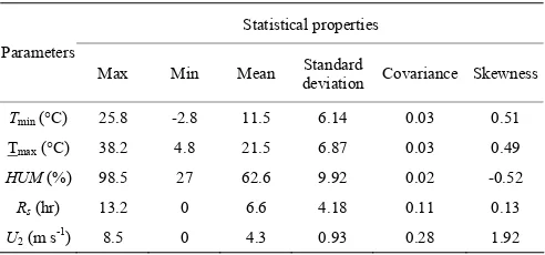
The weather data were collected from the Islamic Republic of Iran Meteorological Organization (IRIMO) (www.weather.ir). The data included the mean, maximum and minimum air temperatures, relative humidity, wind speed, solar radiation and sunshine hours for the period 2003-2011. Table 1 shows some statistical data properties used in this study.
Table 1 Some statistical properties of data
Statistical properties Parameters
Max Min Mean Standard deviation Covariance Skewness
Tmin (°C) 25.8 -2.8 11.5 6.14 0.03 0.51
Tmax (°C) 38.2 4.8 21.5 6.87 0.03 0.49
HUM(%) 98.5 27 62.6 9.92 0.02 -0.52
Rs (hr) 13.2 0 6.6 4.18 0.11 0.13 U2 (m s-1) 8.5 0 4.3 0.93 0.28 1.92
2.2 Climate based methods
The PMF-56 model was utilized to assess the temperature and radiation-based equations. The PMF-56
model assumes the ET0 as that from a hypothetical crop
with an assumed crop height (0.12 m) and fixed canopy
resistance (70 s m-1) and albedo (0.23), closely
approximating the evapotranspiration from an extensive surface of green grass cover of uniform height, actively growing, and with no water shortage, which is given by (Allen et al., 1998) as follows:
[
]
20
2
0.408 ( ) 890 / ( 273) ( )
(1 0.34 )
n mean s a
R G T U e e
ET
U
Δ − + + −
=
Δ + +
γ γ
(1)
where, ET0 is the reference crop evapotranspiration
(mm day-1); Rn is the net radiation (MJ m-2 d-1); G is the
soil heat flux (MJ m-2 d-1); γis the psychometric constant (KPa °C -1); es is the saturation vapor pressure (kPa); ea is
the actual vapor pressure (kPa), and Δ is the slope of the
saturation vapor pressure–temperature curve (kPa oC-1);
Tmean is the daily mean air temperature (°C), and U2 is the
mean daily wind speed at 2 (m ms-1). The data required
for calculating ET0 followed the method and procedure
provided in Chapter 3 of FAO-56 (Allen et al., 1998).
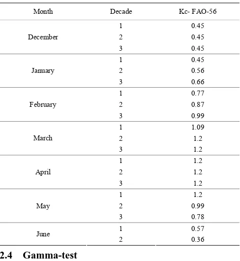
2.3 Crop coefficient
Under standard conditions, the crop evapotranspiration
denoted as ETc, is the evapotranspiration from
data for different crops, the PM method is applied to the estimation of the standard reference crop to verify its evapotranspiration rate, i.e., ET0. The ratios of ETc ET0-1
determined in the experiment was called crop coefficients (Kc), are applied to relate ETc to ET0 or:
ETc=Kc. ET0 (2)
Attributable to discrepancies in the crop
characteristics throughout its growing season, Kc is the
given crop changes from sowing to harvest. The amounts
of crop coefficients under standard conditions (ETc) are
given in Table 2.
Table 2 Crop coefficients
Month Decade Kc- FAO-56
1 0.45 2 0.45 December
3 0.45 1 0.45 2 0.56 January
3 0.66 1 0.77 2 0.87 February
3 0.99 1 1.09 2 1.2 March
3 1.2 1 1.2 2 1.2 April
3 1.2 1 1.2 2 0.99 May
3 0.78 1 0.57 June
2 0.36
2.4 Gamma-test
The gamma-test (GT) measures the minimum mean square error (MSE) that can be realized when modeling the hidden data employing any continuous nonlinear models. The GT was first stated by Koncar (1997) and Agalbjorn et al. (1997), and later improved and discussed in detail by several researchers (Chuzhanova et al., 1998; De Oliveira, 1999; Tsui, 1999; Tsui et al., 2002; Durrant, 2001; Jones et al., 2002).
Simply, a concise introduction to the GT is presented here. The primary notion is quite distinctive from earlier challenges with nonlinear analysis. Assume that we have a group of data observations of the form:
{(xi, yi), 1≤i≤M} (3)
Where the input vectors xi∈Rm are vectors confined to
some closed bounded set C∈Rm and, without the loss of
generality, the equivalent outputs yi∈R are scalars. The
vectors x contains predicatively useful factors influencing
the output y. The only assumption made is that the
underlying relationship of the system has the following form:
y=f(x1, x2…xm) +r (4)
where, f is a smooth function and r is a random variable
that represents noise. Without loss of generality, it can be
expected that the mean of the distribution of r is zero
(since any constant bias can be subsumed into the
unknown function f) and that the variance of the noise
Var (r) is bounded. The domain of a possible model is
now limited to the class of smooth functions which have bounded first partial derivatives. The Gamma statistic Γ is an estimate of the model output variance that cannot be accounted by a smooth data model.
The GT is based on N [i, k], which is the kth (1≤k≤p)
nearest neighbors xN [i, k] (1≤k≤p) for each vector xi (1≤i
≤M). Specifically, the GT is derived from the Delta
function of the input vectors:
2
( , ) 1
1
( ) M
M N i k i
i
k x x
M =
=
∑
−δ 1≤k≤p (5)
where, |...| denotes Euclidean distance, and the corresponding Gamma function of the output values:
2
( , ) 1
1 ( )
2
M
M N i k i
i
k y y
M =
=
∑
−γ 1≤ ≤k p (6)
where, yN(i,k) is the corresponding y-value for the kth
nearest neighbor of xi in Equation (5). In order to
compute Γ a least squares regression line is constructed
for the p points (δ(M, k),γ(M, k))
γ=Aδ+Γ (7) The graphical output of this regression line (Equation (7)) provides very useful information. First, it is
significant that the vertical intercept Γ of y (or gamma)
axis suggests an estimate of the best attainable MSE applying a modeling technique for unknown smooth functions of continuous variables (Evans and Jones, 2002). Second, the gradient offers an indication of the model complexity (a steeper gradient indicates a model of greater complexity).
2.5 Artificial neural network
forms may be pure data or the input results of other neurons, and the output forms may be the results of the final process or the input data of other neurons (Kim and Kim, 2008). Figure 2 is a general architecture of a feed forward neural network. This network comprises of one input layer, one or several hidden layers, and one output layer. Its learning algorithm is back-propagation (BP). In the case of the BP algorithm, first the output layer weights are updated. For each neuron of the output layer, a desired value exists. By this value and the learning rules, the weight coefficient is updated (Adineh et al., 2008). There are several features in ANN that distinguished it from the empirical models (Moghaddamnia et al., 2009). First, neural networks have flexible nonlinear function mapping capability that can approximate any continuous measurable function with arbitrarily desired accuracy, whereas most of the commonly used empirical models do not have this property. Second, being nonparametric and data-driven, neural networks impose few prior assumptions on the underlying process, from which data are generated. Also, high computation rate, learning ability through pattern presentation, prediction of unknown patterns, and flexibility affronts for noisy patterns are other advantages of using ANNs (Adineh et al., 2008). In this study, several architectures and various neurons with two transfer functions embedded in the neural networks were adapted.
Figure 2 Architecture of adaptive neuro-fuzzy inference system
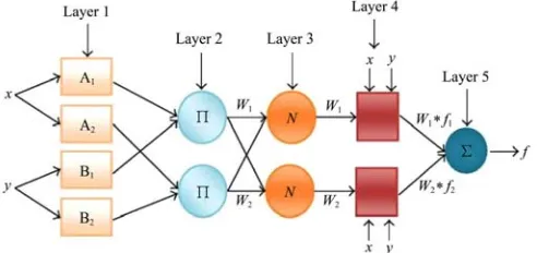
2.6 Adaptive neuro-fuzzy inference system
The ANFIS is a universal estimator and is able to approximate any real continuous function on a compact set to any degrees of accuracy (Jang et al., 1997). The basic structure of the type of fuzzy inference system could be as a model that maps input characteristics to input membership functions. Then, it relates input membership function to rules and the rules to a set of
output characteristics. Finally, it maps output characteristics to output membership functions, and the output membership function to a single output or a decision associated with the output (Jang et al., 1997). Each fuzzy system contains three main parts of fuzzifier, fuzzy database and defuzzifier. Fuzzy database includes two main parts of fuzzy rule base, and inference engine. Figure 3 represents a typical ANFIS architecture. In layer one, every node is an adaptive node with a node function such as a generalized bell membership function or a Gaussian membership function. In layer two, every node is a fixed node representing the firing strength of each rule, and is calculated by the fuzzy and connective of the ‘product’ of the incoming signals. In layer three, every node is a fixed node representing the normalized firing strength of each rule. The i-th node calculates the ratio of the i-th rule firing strength to the summation of two rules firing strengths. In layer four, every node is an adaptive node with a node function indicating the contribution of i-th rule toward the overall output. In layer five, the single node is a fixed node indicating the overall output as the summation of all incoming signals (Jang et al., 1997).
Figure 3 Structure of forecast strategy
2.7 Wavelet Transform
The wavelet transform of a signal is capable of providing time and frequency information simultaneously, hence providing a time–frequency representation of the signal. To accomplish this task, the data series is broken down by the transformation into its wavelets, which are a scaled and shifted version of the mother wavelet (Nason and Von Sachs, 1999). The continuous wavelet transforms (CWT) of a signal x(t) is defined as follows:
* ,
1
( , ) ( ) ( )
| |
s S
CWT s s t t dt
s
=
∫
ψ
τ
τ ψ (8)
where, s is the scale parameter; τ is the translation
parameter and the ‘*’ denotes the complex conjugate. Here, the concept of frequency is replaced by that of scale,
determined by the factor s. ψ(t) is the transforming
function, and is called the mother wavelet. The term wavelet means small wave. The smallness refers to the condition that the function is of a finite length. The wave refers to the condition that it is oscillatory. The term mother implies that the functions used in the transformation process are derived from one main function, the mother wavelet. The wavelet coefficient
CWTψ
x (τ, s) is large when the signal x(t) and the wavelet
ψ*(t–τ s-1) are similar; thus, the time series after the wavelet decomposition allows one to have a look at the signal frequency at different scales. The CWT calculation requires a significant amount of computation time and resources. Conversely, the discrete wavelet transforms (DWT) allows one to reduce the computation time, and is considerably simpler to implement than the CWT.
DWT scales and positions are usually based on the powers of two– the so-called dyadic scales and positions. This is achieved by modifying the wavelet representation
to:
0 0 ,
0 0
1
( ) ( )
| |
j
j k j j
t k s t
s s
−
= τ
ψ ψ (9)
where, j and k are the integers and s0>1 is a fixed dilation
step. The translation factor so depends on the dilation step. The effect of discretizing the wavelet is that the time–space scale is now sampled at discrete intervals. A value of s0=2 is usually chosen so that the sampling of the
frequency axis corresponds to dyadic sampling. This is a very natural choice, for example, for computers, the
human ear and music. A translation factor of s0=1 was
chosen so that there is also dyadic sampling of the time axis. High pass and low pass filters of different cutoff frequencies are used to separate the signal at different scales. The time series is decomposed into one containing its trend (the approximation) and one containing the high frequencies and the fast events (the detail). The scale is changed by above sampling and lower sampling operations. The filtering procedure is repeated every time when some portions of the signal corresponding to some frequencies are removed, obtaining the approximation and one or more details, depending on the chosen decomposition level (Noori et al., 2009).
As depicted in Figure 4, wavelet techniques are implemented in the first and last stages. The actual time-series are first decomposed into a number of wavelet coefficient signals and one approximation signal. The decomposed signals are then fed into the ANFIS at the second stage to predict the future time-series patterns for each of the signals. Finally, the predicted signals are recombined in the last stage to form the final predicted series.
2.8 Data preprocessing
Various input combinations of data were explored in this study to assess their influence on the evapotranspiration modeling (Table 3). The best one can be specified by observing the Gamma value, indicating a measure of the best root mean square error (MSE) possible by applying any modeling methods for unseen continuous variables smooth functions. In Table 3, some very interesting variations of the best MSE are observed with different input combinations. The minimum value of Gamma was observed when all available input data sets were used, i.e. Tmax, Tmin, HUM, Rs and U2. The results of
these tests reveal that the rate of evapotranspiration solar radiation is the most sensitive parameter, because by the removal of these data as an input, the gamma statistic will have the highest value.
Table 3 Gamma test results on different inputs
Input models combinations Gamma RMSE
Tmin, Tmax, HUM, Rs, U2 0.006528 0.000504
Tmin, Tmax, Rs, U2 0.009502 0.00078
Tmin, Tmax, HUM, Rs 0.010069 0.00068 Tmin, HUM, Rs, U2 0.010279 0.0011
Tmax, HUM, Rs, U2 0.012237 0.00098
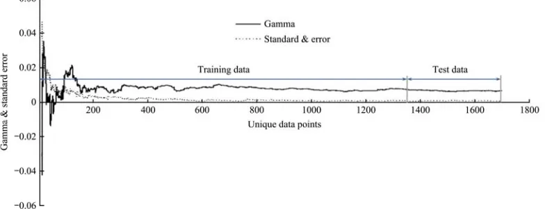
Tmin, Tmax, HUM, U2 0.021697 0.00099 The quantity of available input data to anticipate the desirable output was evaluated using the M-test. The M-test results help to determine whether there were sufficient data to provide an asymptotic Gamma estimate and subsequently a reliable model. The M-test analysis results are presented in Figure 5. As it can be witnessed from the figure, the data standard error for 1360 numbers is the lowest. This number has been selected as the training network data number. The remaining data were used to test the model and estimate the results.
Figure 5 Scatter and time series plots of observed versus estimated wheat evapotranspiration values using ANN
2.9 Performance criteria
First, the normalization on the data is done in line with the following expression. There are two main advantages to normalize features before applying AI methods for prediction. One advantage is to avoid using attributes in greater numeric ranges that control those in smaller numeric ranges, and another advantage is to avoid numerical difficulties during the calculation. It is recommended to linearly scale each attribute to the range (–1, 1) or (zero, 1). In the modeling process, all data values are scaled to the range between zero and 1 as follows: max min 0.5 0.5 n X X X X X ⎛ − ⎞ = + ⎜ ⎟ −
⎝ ⎠ (10)
where, Xn is normalization and X is actual value, but X
is data average and Xmax and Xmin are the maximum and
minimum measurement values.
The performance of AI models for estimating the
daily ETc was evaluated using a wide variety of standard
statistics index. A total of three different standard statistics indexes were employed including the coefficient of determination (R2), RMSE, and Nash Sutcliffe coefficient
(CNS) (Nash and Sutcliffe, 1970; Committee, 1993).
2 1 2 2 2 1 1 ( )( ) ( ) ( ) n
i i p p
i
n n
i i p p
i i
ET ET ET ET
R
ET ET ET ET
= = = ⎡ − − ⎤ ⎢ ⎥ ⎣ ⎦ = − ⋅ −
∑
∑
∑
(11)2
1( )
n i
i ET ETp
RMSE
n
= −
=
∑
(12)2 1 2 1 ( ) 1 ( ) n i p i NS n i i i ET ET C ET ET = = − ∑ = − ∑ − (13)
where, ETi and ETp are the observed and predicted at time
i, respectively; ETi and ETpare the observed and
predicted means at time I respectively; and n is the
number of data points.
3 Results and discussion
3.1 ANN results
an input layer with 5 variables, a hidden layer (with 1 to 40 neurons) and an output layer. The activity functions of sigmoid and tan sigmoid is proposed in this study. To
assess the inclusive data and the predicted results, ET =
f(Tmax, Tmin, HUM, Rs, U2) model were used as an input
for the system. In this study, the combinations of input data are separated into two types (training (80% of data) and testing (20% of data)) before entering the network. The number of hidden layers was varied, as well as the neuron numbers and activation function in each layer. A summary with the statistics performance index and MSE
obtained during the training and testing phases is given in Table 4. Table 4 presents training and testing for neural network model with both sigmoid and tan sigmoid activity function and the best architecture of network with each activity function. The performance statistics results of sigmoid activity function were 0.874, 0.958, 0.259, while the results of tan sigmoid activity function were
0.918, 0.967 and 0.246 for CNS, R2, and RMSE,
respectively. This result indicates the superiority of neural network with tan sigmoid activity function with 1-12-1 architecture and 12 neurons in hidden layer.
Table 4 Architectures of the tested neural networks with their respective performance index
RMSE R2 C
NS Transfer Functions Hidden layers neural epochs architecture Network
train test train test train test tan sigmoid 12 14 1-12-1 0.2618 0.2461 0.985 0.967 0.951 0.918
Sigmoid 15 25 1-15-1 0.2778 0.2586 0.972 0.958 0.866 0.874
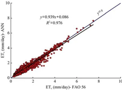
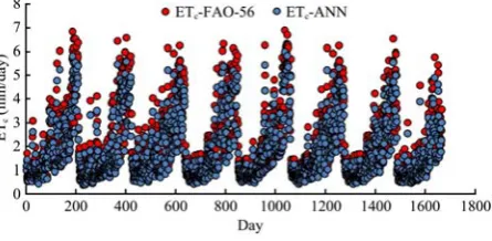
Figure 6 and Figure 7 demonstrates high correlation between FAO-56 measurements and ANN results. The figure indicates that the slope and intercept of the regression equations for ANN model are significantly near to one and zero, respectively. Results obtained from ANN in estimation wheat evapotranspiration indicate high accuracy.
Figure 6 Scatter and time series plots of observed versus estimated values of wheat evapotranspiration from ANN for the
testing data and training data
Figure 7 Scatter and time series plots of observed versus estimated values of wheat evapotranspiration from ANFIS for the
testing data and training data
3.2 ANFIS results
In current study, the architecture of ANFIS with six MFs (membership functions) such as triangular, trapezoidal, bell-shaped Gaussian and Gaussian2 and PI as an input model were used. Also, the MF number was various between two to four. The ideal iterations number was obtained from trial and error procedure. The final structural design and performance statistics of the ANFIS models for the train and test phase are specified in Table
4. Two to six MFs were found to be sufficient for the ET0
estimation using the triangular, trapezoidal, bell-shaped Gaussian and Gaussian2 and PI as an input model, respectively. Moreover, the trapezoidal function was the best MF for almost all the ANFIS models. As presented in Table 5, the trapezoidal function with inputs of the highest and lowest air temperature, solar radiation, relative humidity and wind speed had the greatest performance (CNS = 0.934, R2 = 0.976 and RMSE = 0.039)
among the ANFIS membership functions during test. By considering each MF, ANFIS with a trapezoidal input and 4 MF number was the best model. Also, Figure 8 represents scatter plot, scatter diagram and time series of ANFIS model throughout trapezoidal membership function training and testing.
In Figure 9, although the results gained from ANFIS
model for estimating ETc are acceptable, this superiority
can be demonstrated based on the regression equations
Keskin et al., 2009).
Table 5 Results obtained from different types of ANFIS structures and their performance evaluation
CNS R2 RMSE
MF OPM Epoch
Test Training Test Training Test Training
Trimf 2 6 0.918 0.963 0.929 0.973 0.046 0.015
Trapmf 4 12 0.934 0.971 0.976 0.982 0.039 0.015
Gbellmf 4 26 0.906 0.955 0.898 0.954 0.053 0.013
Gaussmf 2 19 0.926 0.968 0.931 0. 968 0.047 0.013
Gauss2mf 2 15 0.811 0.946 0.809 0.941 0.088 0.028
PImf 3 24 0.856 0.941 0.889 0.923 0.057 0.028
Figure 8 Scatter and time series plots of observed versus estimated values of wheat evapotranspiration from ANFIS for the
testing data and training data
Figure 9 Time series of wheat evapotranspiration during test
3.3 Wavelet-ANFIS results
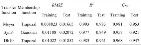
In this section, at first the time series is separated into one comprising its trend (the approximation) and one encompassing the high frequencies and the fast events (the detail). Meyer, Symlet and Daubechies wavelets were used at this stage which is depicted in Figure 10 and Figure 11. The scale is changed by above sampling and lower sampling operations. The filtering procedure is replicated every time when some portions of the signal analogous to some frequencies are removed, obtaining the approximation and one or more details, counting on the selected decomposition level. The selection of appropriate wavelet and the decomposition levels number is highly imperative in data analysis by means of the WT. The number of decomposition levels is selected in terms
of the signal dominant frequency components. The levels are selected so that those parts of the signal that associate well with the frequencies which are needed for classification of the signal are retained in the wavelet coefficients. Then, each of the two parts is conducted separately into the ANFIS prediction model. Table 6 depicts the results of Wavelet-ANFIS. Trapezoidal member functions combination with Mayer wavelet had
the best performance (CNS = 0.953, R2 = 0.983 and
RMSE = 0.0166) during test.
(a) Part approximation
(b) Part Details
Figure 10 Time-series plot of wheat evapotranspiration during test stage using wavelet transform
Figure 11 Scatter and time series plots of observed versus estimated values of wheat evapotranspiration from Wavelet-ANFIS
Table 6 Results obtained from different types of ANFIS-wavelet structures and their performance evaluation
RMSE R2 C
NS Transfer
function
Membership function
Training Test Training Test Training Test
Meyer Trapozal 0.008823 0.01665 0.993 0.983 0.981 0.953 Sym4 Gaussian 0.01188 0.02072 0.977 0.949 0.957 0.921 Db10 Trapozal 0.01022 0.01852 0.983 0.961 0.968 0.947
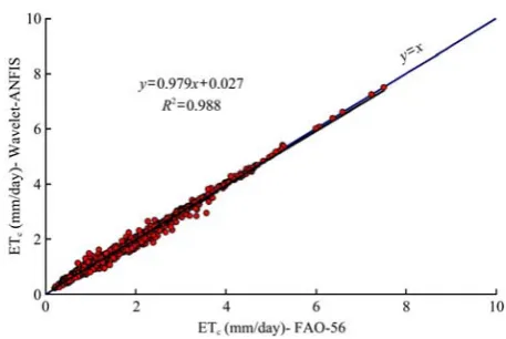
In Figure 12, although the results attained from
Wavelet-ANFIS model for estimating ETc are more
acceptable than other methods, this figure also represents a fit estimated to the observed scattering and time series data and the superior model of prediction.
Figure 12 Scatter and time series plots of observed versus estimated values of wheat evapotranspiration from Wavelet-ANFIS
for the testing data and training data
3.4 Validation performance of models
Being revealed in the results, R2, RMSE and CNS
efficiency coefficient model were applied to compare the performance of models and select the best one. The outcomes of this assessment were presented in Table 7.
Table 7 Values of performance evaluation of three models
Model CNS R2 RMSE
ANN 0.935 0.967 0.2539 ANFIS 0.947 0.949 0.03 Wavelet-ANFIS 0.976 0.988 0.0124
Table 6 shows the best ANN, ANFIS, and Wavelet-ANFIS model anticipation and the data observed to estimate ETc. As witnessed, the CNS and R2 increased
from 0.935 to 0.967 and 0.976 to 0.988, respectively, and
RMSE has declined from 0.2539 to 0.0124. It was
determined that Wavelet-ANFIS hybrid model forecasted evapotranspiration more accurately compared to ANN and ANFIS. In fact, Wavelet-ANFIS models are artificial neural networks, fuzzy logic and wavelet transform
combination, making them more accurate ETc
modeling.
4 Conclusion
The applicability of ANN, ANFIS, and Wavelet-ANFIS approaches in modeling reference evapotranspiration was examined in this article. The daily climatic data from Dashtenaz stations (eight stations), Iran, were used as inputs to artificial intelligent models
for assessing ETc obtained using the standard FAO-56
Penman–Monteith equation and test results were contrasted with each other. Also, Gamma-test and M-Test were determined correspondingly for best combination of input data for measuring and testing computational models. ETc= f(Tmax, Tmin, HUM, Rs, U2) models were
applied as an input model of computational methods. This model includes the highest and lowest air temperature, solar radiation, relative humidity and wind speed from 2003 to 2011. Also, R2, RMSE and CNS model efficiency
coefficient were utilized to compare the performance of models and decide on the best one. The results obtained
with the ANFIS-Wavelet model for ETc estimation were
better than ANN and ANFIS models and confirmed the
capacity of this technique to provide useful tool in ETc
modeling because random weather signals with wavelet decomposition result in reduction of noise and smoothing
these signals. Results indicated that the CNS and R2
increased from 0.935 to 0.967 and from 0.976 to 0.988,
respectively, and RMSE has declined from 0.2539 to
0.0124 after using ANFIS-Wavelet method. This indicates the significance of the wavelet transform in various engineering fields, especially when time series prediction is non-stationary. The study presented methodology is general and if it is the accessible data with high range periods, the methodology can be employed in predicting longer time in the future.
References
Abyaneh, H. Z., A. M. Nia, M. B. Varkeshi, S. Marofi, and O. Kisi. 2010. Performance evaluation of ANN and ANFIS models for estimating garlic crop evapotranspiration. Journal of Irrigation and Drainage Engineering, 137(5): 280–286.
test. Neural Computing and Applications, 5(3): 131–133. Allen, R. G., L. S. Pereira, D. Raes, and M. Smith. 1998. Crop
evapotranspiration-guidelines for computing crop water requirements-FAO Irrigation and drainage paper 56. FAO, Rome, 300(9): D05109.
Aytek, A. 2009. Co-active neurofuzzy inference system for evapotranspiration modeling. Soft Computing, 13(7): 691–700. Benli, B., A. Bruggeman, T. Oweis, and H. Üstün. 2010.
Performance of penman-monteith FAO56 in a semiarid highland environment. Journal of Irrigation and Drainage Engineering, 136(11): 757–765.
Chauhan, S., and R. Shrivastava. 2009. Performance evaluation of reference evapotranspiration estimation using climate based methods and artificial neural networks. Water Resources Management, 23(5): 825–837.
Chiew, F., N. Kamaladasa, H. Malano, and T. McMahon. 1995. Penman-Monteith, FAO-24 reference crop evapotranspiration and class-A pan data in Australia. Agricultural Water Management, 28(1): 9–21.
Chuzhanova, N. A., A. J. Jones, and S. Margetts. 1998. Feature selection for genetic sequence classification. Bioinformatics, 14(2): 139–143.
Committee, A. T. 1993. The ASCE task committee on definition of criteria for evaluation of watershed models of the watershed management committee Irrigation and Drainage Division, Criteria for evaluation of watershed models. Journal of Irrigation and Drainage Engineering, 119(3): 429–442. De Oliveira, A. G. 1999. Synchronisation of chaos and applications
to secure communications. Ph.D. diss., Imperial College of Science, Technology and Medicine, University of London. Durrant, P. J. 2001. WinGamma TM: a non-linear data analysis and
modelling tool with applications to flood prediction. PhD thesis, Department of Computer Science, Cardiff University, Wales, UK.
Evans, D., and A. J. Jones. 2002. A proof of the gamma test. In Proceedings of the Royal Society of London A: Mathematical, Physical and Engineering Sciences, The Royal Society, 2759–2799. London: 2002.
Garcia, M., D. Raes, R. Allen, and C. Herbas. 2004. Dynamics of reference evapotranspiration in the Bolivian highlands Altiplano. Agricultural and Forest Meteorology, 125(1): 67–82.
Gavilán, P., I. Lorite, S. Tornero, and J. Berengena. 2006. Regional calibration of Hargreaves equation for estimating reference ET in a semiarid environment. Agricultural Water Management, 81(3): 257–281.
Gocic, M., and S. Trajkovic. 2010. Software for estimating reference evapotranspiration using limited weather data. Computers and Electronics in Agriculture, 71(2): 158–162.
Jang, R., T. Sun, and E. Mizutani 1997. Neuro-fuzzy and soft
computing; a computational approach to learning and machine intelligence. Englewood Cliffs, NJ: Prentice-Hall.
Jones, A. J., A. Tsui, and A. De. Oliveira. 2002. Neural models of arbitrary chaotic systems: construction and the role of time delayed feedback in control and synchronization. Complexity International, 9: 1–9.
Keskin, M. E., Ö. Terzi, and D. Taylan. 2009. Estimating daily pan evaporation using adaptive neural-based fuzzy inference system. Theoretical and Applied Climatology, 98(1-2): 79–87. Kim, S., and H. S. Kim. 2008. Neural networks and genetic
algorithm approach for nonlinear evaporation and evapotranspiration modeling. Journal of Hydrology, 351(3): 299–317.
Kişi, Ö. 2006. Evapotranspiration estimation using feed-forward neural networks. Hydrology Research, 37(3): 247–260. Kişi, Ö. 2007. Streamflow forecasting using different artificial
neural network algorithms. Journal of Hydrologic Engineering, 12(5): 532–539.
Koncar, N. 1997. Optimisation methodologies for direct inverse neurocontrol. Ph.D. diss., Department of Computing, Imperial College of Science, Technology and Medicine, University of London.
Moghaddamnia, A., M. G. Gousheh, J. Piri, S. Amin, and D. Han. 2009. Evaporation estimation using artificial neural networks and adaptive neuro-fuzzy inference system techniques. Advances in Water Resources, 32(1): 88–97.
Nash, J. E., and J. V. Sutcliffe. 1970. River flow forecasting through conceptual models part I—A discussion of principles. Journal of Hydrology, 10(3): 282–290.
Nason, G. P., and R. V. Sachs. 1999. Wavelets in time-series analysis. Philosophical Transactions of the Royal Society of London A: Mathematical, Physical and Engineering Sciences, 357(1760): 2511–2526.
Noori, R., M. A. Abdoli, A. Farokhnia, and M. Abbasi. 2009. Results uncertainty of solid waste generation forecasting by hybrid of wavelet transform-ANFIS and wavelet transform-neural network. Expert Systems with Applications, 36(6): 9991–9999.
Pereira, A. R., L. R. Angelocci, and P. C. Sentelhas. 2002. Agrometeorologia sfundamentose aplicacoes práticas, Guaíba, Agropecuária. Lavras: Agropecuária.
Sabziparvar, A. A., H. Tabari, A. Aeini, and M. Ghafouri. 2010. Evaluation of class a pan coefficient models for estimation of reference crop evapotranspiration in cold semi-arid and warm arid climates. Water Resources Management, 24(5): 909–920. Sentelhas, P. C., T. J. Gillespie, and E. A. Santos. 2010. Evaluation
Tabari, H., O. Kisi, A. Ezani, and P. H. Talaee. 2012. SVM, ANFIS, regression and climate based models for reference evapotranspiration modeling using limited climatic data in a semi-arid highland environment. Journal of Hydrology, 444: 78–89.
Trajkovic, S. 2005. Temperature-based approaches for estimating reference evapotranspiration. Journal of Irrigation and Drainage Engineering, 131(4): 316–323.
Trajkovic, S., B. Todorovic, and M. Stankovic. 2003. Forecasting of reference evapotranspiration by artificial neural networks. Journal of Irrigation and Drainage Engineering, 129(6): 454–457.
Traore, S., M. Wang, and T. Kerh. 2010. Artificial neural network for modeling reference evapotranspiration complex process in Sudano-Sahelian zone. Agricultural Water Management, 97(5): 707–714.
Tsui, A. P., A. J. Jones, and A. G. D. Oliveira. 2002. The
construction of smooth models using irregular embeddings determined by a gamma test analysis. Neural Computing and Applications, 10(4): 318–329.
Tsui, A. P. M. 1999. Smooth data modelling and stimulus-response via stabilisation of neural chaos, Ph.D. diss., Department of Computing, Imperial College of Science, Technology and Medicine, University of London.
Walter, I. A., R. G. Allen, R. Elliott, M. Jensen, D. Itenfisu, B. Mecham, T. Howell, R. Snyder, P. Brown, S. Echings, T. Spofford, M. Hattendorf, R. Cuenca, J. Wright, and D. Martin. 2000. ASCE’s standardized reference evapotranspiration equation. In: Proceedings of Fourth National Irrigation Symposium, ASAE, Phoenix, AZ, USA, 14–16 November. Zanetti, S., E. Sousa, V. Oliveira, F. Almeida, and S. Bernardo. 2007.