Optimization Algorithm for Lifetime of Mobile Wireless
Sensor Networks Based on Grid
https://doi.org/10.3991/ijoe.v15i01.9778
Ren Song
Jilin University of Finance and Economics, Jilin, China
Abstract—To avoid premature failure due to excessive energy consumption of some nodes in the network, the node energy consumption problem was considered. Network life was maximized. For the problem of node energy consumption, multiple methods such as the shortest path method, optimization method, and power control method were used to solve the problem of optimization of the survival time of the wireless sensor network in different scenarios and improve the network lifetime. The results showed that the sub-gradient algorithm could balance the node energy consumption and the number of neighbor nodes and extend the maximum network lifetime. Therefore, under certain conditions, the algorithm is better than the algorithm using fixed transmission power.
Key Words—Mobile wireless sensor network, network life time, optimization method
1
Introduction
Catalogues of Independent Intellectual Property Rights in Zhejiang Province”, wireless sensor network is one of the key points of development in the next 15 years. In the “Eleventh Five-Year Plan” of the information industry in Hangzhou, the wireless sensor network was included in the “8+1” key industry development target. The National Radio Management Committee passes the dedicated frequency band (779MHz band) of China's wireless sensor network products. In 2007, the National Information Standards Committee established the China Wireless Sensor Network Standard Project Team and began to study the protocol standards for wireless sensor networks. The concept of "perceived China" was promoted by Chinese Premier Wen Jiabao in 2009. Wireless sensor networks play an important role. According to the IDATE report, the global “physical interconnection” business based on wireless sensor networks has achieved a compound annual growth rate of 49% since 2006. The wireless sensor network industry will develop into the next high-tech market with trillion-dollar industry scale. In short, after entering the 21st century, with the advancement of technologies such as microchip manufacturing technology and wireless communication technology, wireless sensor networks have great commercial value and application potential. It will have a profound impact on human production and life.
In terms of application requirements and network management, all sensor nodes must self-organize, self-manage and self-control to form a wireless network. The energy, processing power and storage resources of the sensing nodes are limited. The time-to-live, energy-saving communication protocols and management services need to be optimized. The general communication protocol includes five layers: an application layer, a transport layer, a network layer, a data link layer, and a physical layer. The research on the survival time optimization problem of five protocol layers is one of the main research directions of wireless sensor networks, which has attracted the attention of many scholars. Therefore, the optimization problem of the lifetime of wireless sensor networks is studied from the shortest path tree, optimization method and power control method of graph theory. The wireless sensor network is proposed to be used in different situations to improve the network survival time.
2
State of the Art
(TPGF) based on geographic location information based on the GPSR (Greedy Perimeter Stateless Routing) algorithm. According to the location information, the TPGF algorithm finds a path that can bypass the hole and selects the minimum hop path to transmit data. Fei et al. [4] pointed out that when the node position is unchanged, the sensor nodes distributed near the Sink node have more data than other nodes. The energy consumption is large and the survival time is limited. As the number of sensing nodes increases, the distribution of energy consumption of nodes in the monitoring area is more uneven, and the problem of energy holes is more serious. Therefore, these algorithms are only applicable to smaller wireless sensor networks.
Tang and Yang [5] considered that the movement of the Sink node is a discrete change. At every turn, only the stop position of the Sink node changes. The data collection problem of the mobile Sink node translates into static data collection problems at different stop position. A survival time optimization model of parameters such as stop position, node energy consumption, node transmission rate, and transmission power is established. However, Naranjo et al. [6] do not consider the data collection during the movement of the Sink node, and only consider the data collection where the Sink node stays at a fixed position. Jia et al. [7] proposed range constrained clustering (RCC). All nodes in the monitoring area are divided into several clusters. The ConcordeTSP solver is used to obtain the optimal moving path for the Sink node to traverse all cluster centers. Guo et al. [8] divided the network into several grids and proposed a grid-based clustering method (GBC). A master cluster head is selected in each grid and is responsible for the communication between the heads of the different grid master clusters. A secondary cluster head is selected to collect data from the sensing nodes within the cluster. Lu et al. [9] determined the stop position of the Sink node. However, data collection during Sink's movement has not been considered. The optimization plan of the algorithm still needs further theoretical analysis. Fan et al. [10] only consider the movement of a Sink node. The Sink node needs to collect data from all sensor nodes in the monitoring area. Therefore, the moving path is long and the data collection delay is large.
3
Methodology
3.1 Routing algorithm related to minimum spanning tree
Both PEDAP and PEDAP_PA algorithms are routing algorithms based on the Prim algorithm. Both routing algorithms use the Prim algorithm to construct a minimum weight spanning tree. All nodes send data to the Sink node along the minimum weight generation tree. The difference between these two algorithms is that in the PEDAP algorithm, the link weight is defined as the energy consumption of the two-node communication. In PEDAP-PA, the link weight is defined as the ratio of the energy consumption of the two-node communication to the remaining energy of the transmitting node.
The PEDAP algorithm defines that the energy consumed by node i to send gbit data to node j is:
(1) The energy consumption for defining node i to send gbit data to the sink node is:
(2) In the formula, Eelec represents the circuit electronic energy consumption when a node transmits or receives unit-bit data. Eamp represents the energy consumption of the wireless signal amplifier. dij represents the distance from node i to node j. dis represents the distance from node i to the sink node.
high residual energy as the parent node, which avoids the consumption of nodes with less energy.
3.2 Energy consumption model
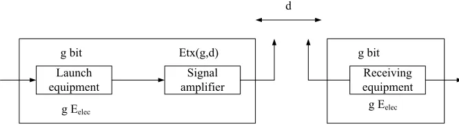
If the wireless channel between the transmitting node and the receiving node is an unobstructed direct path (that is, there are no other obstacles between the two nodes), the transmission power attenuation model of the electromagnetic wave is a power function of the distance between the transmitting node and the receiving node. If there is no barrier-free direct path between the sending node and the receiving node (that is, there are other obstacles between the two nodes), the electromagnetic wave will be reflected between the obstacles and reach the receiving node through different paths in different periods, causing multipath degeneration. The multipath weakened transmission power attenuation model can also be roughly represented by the distance curtain function between the transmitting node and the receiving node. Therefore, at the same received power, the transmit power of the unobstructed direct path and the multipath weakened path increases with the distance between the transmitting node and the receiving node. Block diagram of the AGPS system is shown in Figure 1.
Fig. 1. Block diagram of the AGPS system
Typical wireless sensor network node energy consumption is mainly generated by wireless data transmission and reception. The specific energy consumption model is shown in Figure 1. ETx(g,d) represents the energy consumed by the transmitting node to send gbit data to the receiving node of distance d. ERx(g) represents the energy consumed by the receiving node to receive gbit data. Therefore, the energy consumption ETx(g,d) of the node transmitting module is composed of the transmitting circuit electronic energy consumption ETx-ele and the electronic energy consumption ETx-amp of the signal amplifier portion. The transmission circuit electronic energy consumption ETx-ele is fixed to gEelec. g represents the amount of data sent, and Eelec represents the electronic energy consumption of the circuit when transceiving unit bit data. The electronic energy consumption ETx-amp of the signal amplifier section is related to the node transmission power. A free space model is used. The node adjusts the transmission power at any time according to the communication distance. Therefore, its electronic energy consumption is related to
Launch
equipment amplifierSignal equipmentReceiving
g bit g bit
g Eelec
Etx(g,d)
d
the communication distance. The energy consumption ERx of the receiving module only considers the electronic energy consumption gEelec when receiving the signal.
3.3 Algorithm principle
In a wireless sensor network, a node generally includes a sensing node (referred to as a node) and a sink node (a base station, a data collecting node). In the proposed routing algorithm, there are two assumptions: First, the position of all sensing nodes and Sink nodes is fixed or slowly changing. The mutual location and topology between nodes are not affected, and the Sink node has the entire network topology information. Second, all sensor nodes have the same performance (such as initial energy, energy consumption parameters, maximum transmit power of the node, maximum communication radius, etc.). Third, the transmit power of all sensor nodes varies with the change in communication distance. Fourth, the energy of each sensor node is limited, but the Sink energy is not limited. Fifth, all sensor nodes in the network need to sense and send data. It undertakes data collection and relay tasks and sends data to the Sink node in a direct or multi-hop manner.
In order to avoid excessive loss of energy consumption of the network hub node, the node is divided into two different types of nodes: standard node and warning node according to the remaining energy of the node. The link weights of different types of nodes use different types of weight factors. The specific description is as follows: First, the standard node: if the residual energy value of the node is greater than Cwaning, the node is a standard node. The node prefers to select the surrounding standard nodes to participate in the forwarding of data. Second, the warning node: if the node residual energy value is less than Cwaning, then the node is a warning node. The smaller type weighting factor is used to calculate the link weight around the warning node, and the weight of the link around it is increased, so as to avoid the warning node when transmitting data.
The initial energy of the node is Einital, and the settings of Cwarnig are as follows:
(3)
In the formula, δ is a specific normal number, C(x) is a function of X, and x is a network parameter. The setting of C(X) is as follows:
(4)
approaches |V|, C(x) is infinite. As x increases, Cwarning decreases. When Cwarning is reduced to a certain value, some of the warning nodes are re-established as standard nodes and continue to participate in the routing of data. When x approaches zero, Cwarning approaches zero. At this point, the node below Cwarning is the failed node with energy exhaustion. The declining law of Cwarning accords with the actual situation of the energy of the sensing node. The energy of the starting node is sufficient, and the decreasing speed of Cwarning is relatively fast. However, when the node energy is generally low, the magnitude of the Cwarning decrement becomes slower.
The link weight functions of the LET, Ratio_w, and Sum_w algorithms only consider the size of their own energy. When the link is selected, the remaining energy of the neighbor node is considered, which is beneficial to avoid excessive participation of the node with small remaining energy in data routing. In summary, the remaining energy of the neighbor nodes and the remaining energy of the nodes are considered. The concept of node classification was introduced. A new link weight function is established. A life optimized routing algorithm based on shortest path tree (LORA-SPT) is proposed. Re(i) represents the remaining energy of node i. Re(j) represents the remaining energy of node j. wij represents the weight of the link (i, j). Cij (g,d) represents the energy consumption of the g-bit data transmitted between the sensing nodes i and j. dij represents the distance between node i and section j. After completing the update of the network weight of this round, the Dijkstra algorithm is used to find the shortest path from the source node to the target node, and the shortest path tree is output. According to the link energy consumption, the remaining energy of the node and the remaining energy of the neighbor node, the energy consumption is large and the link of the warning node at the other end is large by the wij. After being calculated by the Dijkstra algorithm, the link may not be added to the shortest path tree. The node generally selects the link with low energy consumption and sends data through the path of the standard node, so that the warning node can be avoided as a hub node, thereby balancing the energy consumption of the node and prolonging the network lifetime.
4
Result Analysis and Discussion
4.1 Algorithm implementation
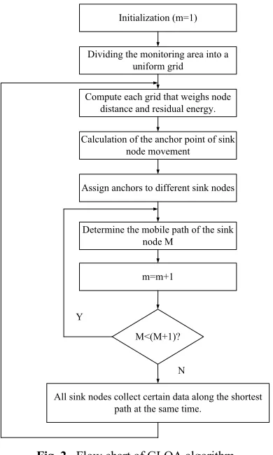
node, the moving path selection model (15) is solved, and the shortest moving path of the sink node is obtained. Sixth, the gateway node notifies the Sink node of the mobility scheme. Sink nodes collect data by static collection or mobile collection along the shortest path. When certain data collection is complete, it returns to step 1. The above steps are performed cyclically until a node is exhausted and fails. Flow chart of GLOA algorithm is shown in Figure 2.
Fig. 2. Flow chart of GLOA algorithm
The time complexity of the GLOA algorithm is analyzed. The time complexity of the algorithm mainly consists of the time complexity determined by the anchor point, the time complexity of the clustering algorithm, the time complexity determined by the moving path, and the time complexity of the data collection algorithm. The anchor point is determined by the fact that each anchor point needs to iteratively calculate the potential value of all the meshes, that is, its time complexity is θ(n2N). The time complexity of the clustering algorithm is the division of the observations of the loop execution and the calculation of the center of the new cluster, that is, , θ(IcM|V|). |V| indicates the number of sensor nodes in the network. Ic represents the number of iterations. The determination of the moving path is to solve the moving path selection
Initialization (m=1)
Dividing the monitoring area into a uniform grid
Compute each grid that weighs node distance and residual energy.
Calculation of the anchor point of sink node movement
Assign anchors to different sink nodes
Determine the mobile path of the sink node M
m=m+1
All sink nodes collect certain data along the shortest path at the same time.
M<(M+1)? Y
model, which is determined by the algorithm used. In order to reduce the time complexity of the algorithm, the GLOA algorithm uses the nearest neighbor insertion method in graph theory to determine the access order of the anchor points. The shortest mesh path between anchors is sought. Finally, an approximate solution of the shortest moving path is obtained. Its time complexity is θ(n(N2+N2+…+N2)). The time complexity of the data collection algorithm is related to the shortest path tree algorithm. If the Bellman-Ford algorithm is used, its time complexity is related to the rate of change of data and path weights of neighbor nodes.
4.2 Algorithm simulation
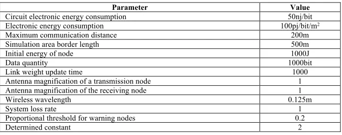
The parameters of the algorithm simulation are shown in Table 1:
Table 1. Simulation parameter table
Parameter Value
Circuit electronic energy consumption 50nj/bit
Electronic energy consumption 100pj/bit/m2
Maximum communication distance 200m
Simulation area border length 500m
Initial energy of node 1000J
Data quantity 1000bit
Link weight update time 1000
Antenna magnification of a transmission node 1
Antenna magnification of the receiving node 1
Wireless wavelength 0.125m
System loss rate 1
Proportional threshold for warning nodes 0.2
Determined constant 2
In general, communication energy consumption is far greater than other energy consumption. Therefore, in the simulation, energy consumption such as calculation, data fusion, information query packet transmission and reception, time-consuming retransmission, error and other energy consumption during data transmission are not considered, and only data wireless communication energy consumption is considered. A 500×500 m2 network simulation area was selected. Within this area, the locations of evenly distributed 30, 40, 50, 60, 70, 80, 90, 100 wireless sensor network nodes (including one Sink node and other sensing nodes) are randomly generated. The Sink node has fixed coordinates (250, 250). In order to verify the effectiveness of the algorithm, for each fixed node number of wireless sensor networks, 10 different network locations of different node locations are randomly generated. According to the simulation parameters of Table 1, the network lifetime, average node energy consumption and node average delay of the 10 different network topologies are calculated respectively. Finally, the average value is taken as the simulation result value of the wireless sensor network performance parameter of the number of nodes.
Average node energy consumption = total energy consumption of all nodes / (number of nodes × DGC number) when the energy of the first node is exhausted. Node average delay = the total number of hops / (number of nodes × DGC) that all nodes send data to the sink node when the first node is exhausted.
4.3 Comparison of algorithm simulation results
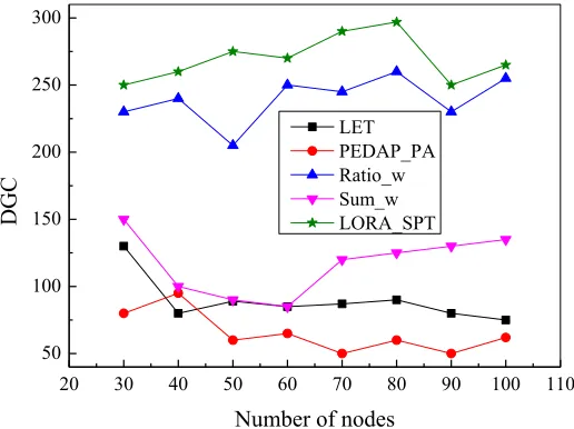
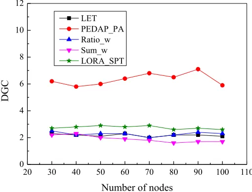
To verify the validity of the algorithm, the LET, PEDAP_PA, Ratio_w, Sum_w, and LORA_SPT algorithms are compared. Comparison of network lifetimes of algorithms is shown in Figure 3.
Fig. 3. Comparison of network lifetimes of algorithms
Figure 3 compares the network lifetime of each algorithm. As shown in Figure 3, the network lifetime (DGC number) of the LORA_SPT algorithm is larger than that of LET, PEDAP_PA, Ratio_w, and Sum_w; the algorithm is optimal, followed by the Ratio_w algorithm. The algorithm considers link energy consumption, energy consumption of its own nodes and energy consumption of neighbor nodes. Type weighting factors are introduced to avoid premature death of nodes with less residual energy (warning nodes) that are too involved in routing data. Therefore, in terms of network lifetime, LORA_SPT extends network lifetime.
The average node energy consumption of each algorithm is compared. The average node energy consumption of the LORA_SPT, LET, Sum_w, and Ratio_4 algorithms is not much different. However, the average node energy consumption of these four algorithms is much lower than the PEDAP_PA algorithm. To avoid warning node energy dying prematurely, the LORA_SPT algorithm avoids the warning node on some path selections and selects a path with relatively large energy consumption. Therefore, in terms of energy consumption, the LORA_SPT algorithm keeps node
20 30 40 50 60 70 80 90 100 110
50 100 150 200 250 300
DGC
Number of nodes
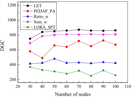
energy consumption to a low level to some extent. Comparison of network lifetimes of algorithms is shown in Figure 4.
Fig. 4. Comparison of network lifetimes of algorithms
When the energy of one node of the network is exhausted, the average remaining energy of other nodes is compared. The node average residual energy of the LORA_SPT algorithm is the lowest, and Ratio_w and PEDAP are the second, but these three algorithms are lower than LET and Sum_w. The LORA_SPT algorithm divides nodes into two types of nodes (standard nodes and warning nodes). The type weight of the warning node is smaller than that of the standard node, and the weight of the surrounding link becomes larger. The warning node can be avoided when the path is selected. Each node selectively participates in network routing based on remaining energy. Therefore, in terms of energy consumption, the LORA_SPT algorithm equalizes the energy consumption of each node of the network. Comparison of residual energy of average nodes of each algorithm is shown in Figure 5.
20 30 40 50 60 70 80 90 100 110
0 2 4 6 8 10 12
D
G
C
Number of nodes
Fig. 5. Comparison of residual energy of average nodes of each algorithm
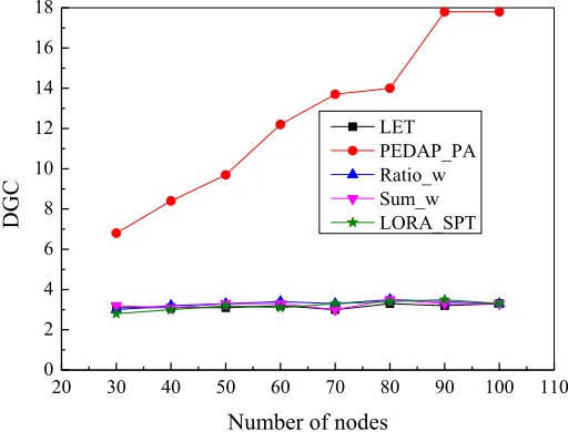
Figure 6 compares the network average delay (hop count) for each algorithm. As shown in Figure 6, the network average delay of the LORA_SPT algorithm is the smallest, and the network average delay of the LET, Sum_w, and Ratio_w algorithms is larger than the LORA_SPT algorithm, but the average delay of these four algorithms is much lower than that of PEDAP_PA. The LORA_SPT algorithm considers the new weight function. Network lifetime is optimized. The node selects the preferred path to send data. To some extent, the average hop count from the node to the sink node is reduced. Therefore, in terms of network delay, the LORA_SPT algorithm reduces the delay of the network. Comparison of average node residual energy of each algorithm is shown in Figure 6.
20 30 40 50 60 70 80 90 100 110
200 400 600 800 1000 1200
DGC
Number of nodes
Fig. 6. Comparison of average node residual energy of each algorithm
In summary, the LORA_SPT algorithm extends the network lifetime, equalizes the energy consumption of each node in the network, and reduces the average network latency (hop count). Node energy consumption is kept at a low level. It is better than the LET, PEDAP_PA, Sum_w, and Ratio_w algorithms.
5
Conclusion
The grid-based survival time optimization algorithm for mobile wireless sensor networks is studied. Firstly, the routing algorithm, energy consumption model and algorithm principle related to the minimum spanning tree are studied. Secondly, using the LORA_SPT algorithm, a weight function based on energy factor, self-node residual energy factor, neighbor node residual energy factor and type weight factor is constructed. The link weights are calculated by using different types of weight factors for different types of nodes. Finally, the Dijkstra algorithm is used to construct the shortest path tree. By adjusting the four factors of the weight function, the LORA_SPT algorithm can prolong the network lifetime, balance the energy consumption of each node of the network, keep the node energy consumption at a low level, and reduce the network average delay (hop count).
The LORA_SPT algorithm is a centralized routing algorithm, which requires nodes to aggregate their information into Sink nodes. When it is uniformly processed by the Sink node, the network topology of other nodes is notified. Centralized routing algorithms can be applied to static wireless sensor networks. However, it does not adapt well to dynamic wireless sensor networks. Simulation experiments show that the optimal life-time distributed routing algorithm based on the shortest path tree can prolong the network lifetime, reduce the network delay, and make the energy
20 30 40 50 60 70 80 90 100 110
0 2 4 6 8 10 12 14 16 18
D
G
C
Number of nodes
consumption economical. Its effect of extending the network lifetime is similar to the LORA_SPT algorithm. When constructing the shortest path tree and calculating the link weight, the optimized lifetime based distributed routing algorithm based on the shortest path tree and the LORA_SPT algorithm use different methods.
6
References
[1]Han, G., Qian, A., Jiang, J., Sun, N., & Liu, L. (2016). A grid-based joint routing and charging algorithm for industrial wireless rechargeable sensor networks. Computer Networks, 101: 19-28 https://doi.org/10.1016/j.comnet.2015.12.014
[2]Rault, T., Bouabdallah, A., & Challal, Y. (2014). Energy efficiency in wireless sensor networks: A top-down survey. Computer Networks, 67: 104-122 https://doi.org/10.1016/j. comnet.2014.03.027
[3]Liu, L., Song, Y., Zhang, H., Ma, H., & Vasilakos, A. V. (2015). Physarum optimization: A biology-inspired algorithm for the Steiner tree problem in networks. IEEE Transactions on Computers, 64(3): 818-831 https://doi.org/10.1109/TC.2013.229
[4]Fei, Z., Li, B., Yang, S., Xing, C., Chen, H., & Hanzo, L. (2017). A survey of multi-objective optimization in wireless sensor networks: Metrics, algorithms, and open problems. IEEE Communications Surveys & Tutorials, 19(1): 550-586
https://doi.org/10.1109/COMST.2016.2610578
[5]Tang, C., & Yang, N. (2017). Virtual grid margin optimization and energy balancing scheme for mobile sinks in wireless sensor networks. Multimedia Tools and Applications, 76(16): 16929-16948 https://doi.org/10.1007/s11042-016-3596-7
[6]Naranjo, P. G. V., Shojafar, M., Mostafaei, H., Pooranian, Z., & Baccarelli, E. (2017). P-SEP: A prolong stable election routing algorithm for energy-limited heterogeneous fog-supported wireless sensor networks. The Journal of Supercomputing, 73(2): 733-755
https://doi.org/10.1007/s11227-016-1785-9
[7]Jia, D., Zhu, H., Zou, S., & Hu, P. (2016). Dynamic cluster head selection method for
wireless sensor network. IEEE Sensors Journal, 16(8): 2746-2754
https://doi.org/10.1109/JSEN.2015.2512322
[8]Guo, S., Wang, C., & Yang, Y. (2014). Joint mobile data gathering and energy provisioning in wireless rechargeable sensor networks. IEEE Transactions on Mobile Computing, 13(12): 2836-2852 https://doi.org/10.1109/TMC.2014.2307332
[9]Lu, X., Wang, P., Niyato, D., Kim, D. I., & Han, Z. (2016). Wireless charging technologies: Fundamentals, standards, and network applications. IEEE Communications Surveys & Tutorials, 18(2): 1413-1452 https://doi.org/10.1109/COMST.2015.2499783
[10]Fan, X., Jia, H., Wang, L., & Xu, P. (2017). Energy Balance Based Uneven Cluster Routing Protocol Using Ant Colony Taboo for Wireless Sensor Networks. Wireless Personal Communications, 97(1): 1305-1321 https://doi.org/10.1007/s11277-017-4567-7
7
Author
Ren Song is a Researcher of Jilin University of Finance and Economics, Jilin, China. His research interests include Optimization Algorithm.