Dynamic Market Participation and Endogenous
Information Aggregation
Edison G. Yu
yFederal Reserve Bank of Philadelphiaz
March 2017
Abstract
This paper studies information aggregation in nancial markets with recurrent in-vestor exit and entry. I consider a dynamic general equilibrium model of asset trading with private information and collateral constraints. Institutional investors can dier in their aversion to Knightian uncertainty: When uncertainty is high, some investors exit the market. Since exiting investors' information is not fully revealed by prices, conditional return volatility and risk premia both increase. I use data on institutional investors' holdings of individual stocks to show that investor exits indeed move nega-tively with price informativeness. The model also implies that exit is more likely when wealth is more concentrated in the hands of less uncertainty-averse investors. The model thus predicts less informative prices toward the end of a long boom, as seen in the data. Moreover, economies with looser collateral constraints should see more volatility due to exit and partial revelation. Higher capital requirements can improve welfare by inducing more information revelation by prices.
I would like to thank Monika Piazzesi and Martin Schneider for the many useful discussions. I also like to
thank Manuel Amador, Marissa Beck, Mitchell Berlin, Jayant Ganguli, Anatasios Karantounias, Siddharth Kothari, Pete Klenow, Pablo Kurlat, Tim Landvoigt, Benjamin Lester, Alejandro Molnar, Muriel Niederle, Rodney Ramcharan, Krishna Rao, Filip Rozsypal, Florian Scheuer, Luke Stein, John Taylor, Peter Troyan, William Gui Woolston, Yaron Leitner, and seminar participants in Stanford University, Federal Reserve Bank of Philadelphia, Federal Reserve Board of Governors, London School of Business, and Melbourne University. This research is funded by the Federal Reserve Bank of Philadelphia.
yFederal Reserve Bank of Philadelphia, Research Department, Ten Independence Mall, Philadelphia, PA
19106-1574. E-mail: [email protected]
zThe views expressed in this paper are those of the author and do not necessarily reect the views of the
1. Introduction
Investors adjust their stock positions at both the intensive and extensive margins. Around 40% of changes in the stock positions of institutional investors in the U.S. are due to changes at the extensive margin.1 Most standard rational expectations models with asymmetric
information do not capture changes in investor participation in equilibrium. In these models, investors respond to signals by adjusting their asset positions only at the intensive margin. However, changes at the extensive margin can have important implications for information aggregation. When investors close out their positions and leave the market as opposed to simply reducing their asset positions, their private signals may not be fully reected in equilibrium prices and thus will be lost. Moreover, the amount of wealth that investors have can also aect their decisions on closing positions. This paper studies information aggregation in a dynamic setting that highlights the important interaction between the changes in the wealth distribution among investors and information aggregation over time. Specically, I nd that a more unequal wealth distribution in favor of the less ambiguity averse investors leads to more information loss.
To study how changes in market participation and the wealth distribution aect informa-tion aggregainforma-tion, I consider a dynamic asset market model that incorporates private signals, ambiguity aversion (or aversion to Knightian uncertainty), logarithmic preferences, and bor-rowing constraints. When investors are ambiguity averse, their private signals may not be fully revealed in equilibrium. Papers by Condie and Ganguli (2011a,b, 2012) show that, in a static setting, private information that is perceived to be ambiguous need not be revealed by market prices in a rational expectations equilibrium. This paper builds an innite horizon dynamic model to study the interaction of wealth distribution dynamics and information aggregation in the long-run. In the model, investors receive private signals about the future payo of risky assets. However, the interpretation of these signals is ambiguous. Specically, potential investors are uncertain about the likelihood function of the true signal-generating process and evaluate probabilities according to the worst case scenario. If the uncertainty regarding the signal interpretation is high, investors may decide not to invest in risky assets. When there is heterogeneity in the level of ambiguity among investors, the more ambiguous investors exit the stock market, and a partially revealing equilibrium exists in which the 1Using 13F ling data on institutional investors' stock positions, I can compute the changes in stock
private signals of these exited investors are not fully revealed. This leads to information loss and higher return volatility of the risky asset.
Why would ambiguity aversion of investors lead to partial revelation of information in equilibrium? In the model, investors make portfolio decisions over purchasing a risk-free bond and a stock. They each receive an independent private signal from a nite state space about the next-period payout of the stock. In a standard rational expectations model, investors hold non-zero amounts of stock in equilibrium except for knife-edge cases. Given prices, their demand for the stock is responsive to the private signal received. A good signal about future payos of the stock leads to more demand for the stock, while a bad signal leads to less demand. In equilibrium, market clearing means that these changes in demand lead to equilibrium prices that are responsive to the signals that investors receive. Investors can therefore infer the private signals of other investors from the equilibrium prices. This leads to a fully revealing equilibrium in which prices reect information from all signals, which has been shown to exist generally in the previous literature.
With ambiguity aversion, however, investors are uncertain about the correct likelihood function of the signal to use for updating their beliefs and instead update their posterior beliefs using a set of likelihood functions, where the size of the set reects the degree of am-biguity. Ambiguity aversion is modeled as in Gilboa and Schmeidler (1989), where investors are averse to the worst case scenario. Specically, when they hold a long position in the stock, investors pick the likelihood function in the set that generates the most pessimistic belief about the payo. For investors to buy the stock, its price must be low enough to be appealing even under the most pessimistic belief. Symmetrically, when they hold a short position in the stock, they pick the likelihood function that leads to the most optimistic belief about the payos, which is the worst case for a short position. Ambiguity aversion thus implies that there is a region of prices where investors choose zero stock. Hence, an investor may stay out of the stock market under dierent realizations of her private signal, and so her demand for stock becomes non responsive to her private signal received.
gives rise to an interesting interaction between the wealth distribution and revelation. When the less ambiguous investor is relatively wealthy, it's more likely that she can purchase all of the stock using her wealth, and this leads to more information loss.
In a static model, one cannot answer the question whether heterogeneity and the wealth distribution matter in the long run. For example, if the long-run wealth distribution becomes degenerate that only investors who are less ambiguous survive, then we can just focus on a model with one representative investor. The heterogeneity in investors becomes unimportant in the long run. The dynamic setup of this paper can help to address these questions because the wealth distribution in this paper is endogenously determined. I nd equilibria where investors of dierent degrees of ambiguity aversion survive in the long-run. Moreover, the model can provide insights about the dynamic interaction of the the relative wealth distribution of the investors and information eciency. In a dynamic setup where investors levels of impatience and ambiguity aversion are positively correlated, the less impatient and ambiguity-averse investors, on average holds more stock. A sequence of good shocks to the stock payos leads these investors to have more wealth relative the less patient and more ambiguity-averse investors. If this is followed by a period of increased uncertainty, partial revelation would occur more often than if the period of increased uncertainty comes after a sequence of bad shocks to the payos of the stock. So the introduction of the dynamics of the wealth distribution generates boom-bust cycles accompanied by endogenous information propagation.
The presence of the wealth eect implies that capital requirements also aects information aggregation in equilibrium. The less ambiguous investor nances part of her purchase of the stock through borrowing. A tighter collateral constraint makes it more dicult for her to purchase all of the stock, and the more making partial revelation less likely. A policy that tightens capital requirement can lead to a welfare gain. The information eciency gain from a stricter capital requirement may outweigh the welfare loss from its distortion of trade.
rst show that more exits of investor from a stock are associated with less informative prices. For example, exits of 10 institutional investor from a stock are associated with a 33 percentage point decrease in the the growth rate of the price informativeness measure. Then the results also suggest that prices are less informative when the share holdings of a stock are more disperse among institutional investors. Last but not least, I show that there is more information loss when a stock is at the end of a long boom. These are all consistent with the model implications.
Related Literature This paper is related to several strands of literature. Early papers like those by Grossman and Stiglitz (1976), Radner (1979), and Allen (1981) study asymmetric information in a general equilibrium setting, usually nding that the existence of a fully revealing equilibrium is generic.2 In particular, Radner (1979) shows that, in a pure exchange
economy with a nite number of signal states, a rational expectations equilibrium reveals to all traders the information possessed by all the traders taken together except for knife-edge cases. This paper shows that, in a setup with a nite set of signals, a rational expectations equilibrium with partial revelation is a robust phenomenon when investors in the economy are ambiguity-averse.
There is also a literature on limited participation. Ambiguity aversion has been considered in problems of portfolio choice. Dow and Werlang (1992) pioneer the idea that ambiguity-averse investors may not hold any risky assets in a static portfolio choice model. Epstein and Schneider (2007) study non participation and market equilibrium in a dynamic setting with ambiguity-averse investors.3 Cao et al. (2005) is a closely related paper that studies
limited participation with model uncertainty but without asymmetric information. Limited participation can also be generated through other mechanisms. Constantinides (1979), Davis and Norman (1990), and Morton and Pliska (1995) show that transaction costs can lead to no-trade regions for risky assets with risk-averse investors.4 Vissing-Jorgensen (2002)
provides empirical evidence that supports the importance of xed transaction costs to explain household non participation in the stock market. Similarly, Reis (2006), Chien et al. (2009), and Due (2010) show in models with rational inattention that investors can also limit their participation in the market. When investors are faced with transaction costs or when they
2Allen and Jordan (1998) provide an excellent survey of this literature.
3Epstein and Schneider (2010) provide a thorough survey of how models with ambiguity-averse investors
can be useful in studying nancial market phenomena.
4A number of other papers, including those by Due and Sun (1990), Heaton and Lucas (1996), Vayanos
are rationally inattentive, they may choose not to re-balance their portfolios in response to shocks. They do not necessarily exit the market during times of uncertainty, however. This paper provides a way to model the time-varying exit behavior through state-dependent ambiguity aversion. The framework of this paper can also be used to model xed holding costs through a simple reinterpretation of the zero-holding region of stock. This paper also studies how limited participation can play an important role in information aggregation, which is not the focus of the earlier papers.
A few papers show that partially revealing equilibria exist in a static setting with ambiguity-averse investors. Condie and Ganguli (2011a,b) demonstrate, in the tradition of Radner (1979), the existence and robustness of partially revealing rational expectations equilibria even in the absence of noise shocks. In another paper with a normal payo distribution, Condie and Ganguli (2012) show that private information that is perceived to be ambiguous need not be revealed by market prices in a rational expectations equilibrium, and nding that the risk premium is higher and price volatility is lower when there is unrevealed infor-mation. Easley et al. (2012) also nd partial revelation in the absence of noise. The mutual fund investors in their paper are not ambiguous over the fundamentals of the stock but over the strategy used by hedge fund managers. This paper complements this literature by study-ing endogenous information aggregation and its interaction with the wealth distribution in a dynamic setting with an innite horizon and nite states. A few recent papers such as Bianchi et al. (2014), Ilut and Schneider (2014), and Ilut et al. (2015) study equilibrium with ambiguity aversion for the broader economy in dynamic settings.
Partial revelation is also possible under alternative models. The noise based approach is a widely used alternative to generate partial revelation. In these models, signal values are not fully revealed in equilibrium due to the presence of noise shocks.5 Dow and Gorton
(2008) provide a recent discussion of this approach. Tallon (1998), Caskey (2009), Mele and Sangiorgi (2009), and Ozsoylev and Werner (2011) nd partial-revelation results with ambiguity-averse investors. The partial revelation in these models relies, however, on the presence of noise in the market. Using a dierent approach, Hong and Stein (2003) show that partial revelation can occur when investors are faced with short-sell constraints in a three-period setting. This paper describes a dynamic model environment when information may not be revealed in the absence of noise trading.
There is a vast literature on heterogeneous beliefs in nancial markets and their impli-5See Grossman and Stiglitz (1980), Hellwig (1980), Diamond and Verrecchia (1981), and Admati (1985),
cation on asset pricing. See Williams (1977), Varian (1989), Abel (1990), Harris and Raviv (1993), Detemple and Murthy (1994), Basak (2000), and Scheinkman and Xiong (2003) for example of earlier work. Basak (2005) provides a survey of this literature.6 Work in this
literature generally nds that heterogeneous agent beliefs and preferences lead to the wealth distribution being an important determinant on asset prices. Heterogeneous beliefs and preferences can also generate time-varying risk premium, higher stock return volatility, and higher trading volume, which help to model various market phenomenon such as the equity premium puzzle (Mehra and Prescott (1985)), excessive volatility (Shiller (1981)), and the leverage eects (Black (1976), Schwert (1989), and Campbell and Lettau (1999)). This pa-per complements the literature by providing a way to study endogenous participation, where agents choose to enter and exit the market dynamically as a function of ambiguity aversion and the endogenous wealth distribution, as oppose to exogenous market participation. The model in this paper can generate time-varying risk premium and higher volatility through the time-varying ability of prices to aggregate information. The increase in risk premium and volatility in this paper is coming from agents' private information not being completely reected in market prices and quantities. This endogenous movement in volatility as a result of information loss is separate from the the higher volatility comes from endogenous asset price movement due to heterogeneous beliefs and preferences.
A large literature has used institutional ownership to examine the relationship between institutional ownership and stock returns. These papers nd a correlation between changes in institutional ownership, stock returns, and return volatility. See Sias (1996), Nofsinger and Sias (1999), Wermers (1999), Dennis and Strickland, 2002, Xu and Malkiel, 2003, Cai and Zheng (2004), Sias et al. (2006), Rubin and Smith, 2009, and Hong and Jiang (2011) for examples.There is also a growing literature that explores what might aect price infor-mativeness. For example, Boehmer and Wu (2013) nd that short-sell activity increases informational eciency, while Fernandes and Ferreira (2009) show that insider trading law helps improve price informativeness. The empirical exercise in this paper also uses data on institutional ownership and a measure of price informativeness based on Chen et al. (2007), but focuses on the interaction between changes in institutional ownership at the extensive margin and stock price informativeness that is implied by the model.
The rest of the paper is structured as follows: Section 2 describes the dynamic model 6For more recent work, see Buraschi and Jiltsov (2006),Li (2007), David (2008), Dumas et al. (2009),
and its computation. Section 3 discusses numerical results of the dynamic model. Section 4 shows welfare calculation. Section 5 presents empirical results using data on stock holdings of institutional investors. Section 6 concludes.
2. The Dynamic Model
The endogenous information revelation in the model is driven by the extensive margin changes in investment by investors with private information. The following setup of the model uses ambiguity aversion as one explanation to the extensive margin changes. It should be emphasized that ambiguity aversion can be replaced with other setups using the frame-work of the paper and the results of the paper remain the same. Fixed holding costs or regulatory constraints, for example, can also lead to extensive margin changes in invest-ment. After describing the setup with ambiguity aversion below, I will show that the setup can be easily applied to modeling xed costs or other constraints with virtually no change.
2.1. Model Environment
There are two assets in the economy, a risk-less bond and a stock. The risk-less bond lives for one period and pays out one unit of consumption. The stock is long-lived and pays a dividend Dtevery period. The dividend grows at a rate gt, which follows an iid process with
mean t and variance 2. The law of motion for the dividend is then Dt = Dt 1egt. Each
period, nature chooses a mean t for the next-period mean growth rate. Investors do not
know tand they need to form beliefs about the distribution of the mean. This setup means
that investors do not know the actual realization of gt even when they know the true t.
There are two investors, A and B, in the model. Each investor receives a private signal si
t , i = A; B each period about the next-period mean growth rate t. The signals sAt and sBt
are generated independently over time and of each other from a nite state space according to the true likelihood function `0(stjt). If there is no ambiguity, a Bayesian investor who
knows both the signals st = (sAt ; sBt ) updates her belief about the distribution of t using
Bayes' rule:
p(tjst) = R `0(stjt)p(t) `0(stjt)p(t)d
, where i = A; B:
An investor who is ambiguous is not sure about the correct likelihood function of the signal. Instead, she perceives a possible set of likelihood functions f`(sj) : ` 2 Lig; i = A; B.
Intuitively, the size of the set Li measures the degree of ambiguity and the subscript i
indicates that the set of likelihood functions can dier between investors. I assume that the true likelihood function is in the set `0 2 Li and that Li to be convex and compact. An
investor updates her beliefs by applying Bayes' rule with each likelihood function in her set Li. If an investor observes both signals, her one-period-ahead posterior distribution set Mi t
is given by
Mi
t fp(tjst)g =
(
`(stjt)p(t)
R
`(stjt)p(t)d
j ` 2 Li
)
, where st= (sAt; sBt ): (1)
This signal structure is similar to those in Epstein and Schneider (2008) and Condie and Ganguli (2012). The posterior under no ambiguity is a special case when Li is a singleton
that contains only the true likelihood `0(stjt). The setup here assumes that ambiguity
is over the interpretation of the signal-generating process rather than over the prior belief on .7 The likelihood function set Li is assumed to be xed over time. This assumption
suggests that the investors' levels of ambiguity do not change over time. Thus an investor with ambiguity aversion believes that the mean dividend growth rate is in the set
fE(tjst)g =
Z
p(tjst)d j p(tjst) 2 M i t
: (2)
Investors can trade on the stock and the bond. They start with initial stock holdings X0
and initial bond holdings B0.8 Investors make consumption and savings/portfolio decisions
to maximize their lifetime utility. Since investors are ambiguity-averse, utility maximization is a max-min problem following the idea in Gilboa and Schmeidler (1989) and can be written as
max
fXi
t+1;Bt+1i ;Citg1t=0
min `2Li ( E` " 1 X t=0
tu(Ci t)jIti
#)
, i = A; B: (3)
Without the min operator, this would become a standard portfolio choice problem. The minimization reects investors' aversion to ambiguity in the sense that they worry about 7We can also obtain sets of posterior distributions if we assume that the ambiguity is over the prior, but
the interpretation would be dierent.
the worst case scenario.9 Investors maximize their expected utility, where the worst case is
dened as minimization over the set Li.10
The information set Ii
t for investor i in equation (3) represents the information she directly
observes and infers from the equilibrium outcomes. For example, when an investor i can observe the signal pair st at time t perfectly, Iti = st; when i can only observe her own
signal but cannot infer any information about the other investor's signal, Ii
t = sit. But
the information set could potentially include the signal of an investor's own signal and information she can partially infer through observing equilibrium prices and quantities. Since the mean dividend growth rate follows an iid process, the signal is only informative for the next-period mean growth rate. Hence, the information set Ii
tis a function of only the
current-period signal and not the whole signal history. This assumption helps to keep the size of the state space manageable.
Investors are subject to a budget constraint
Ci
t+ PtXt+1i +R1 tB
i
t+1 = (Pt+ Dt)Xti+ Bti; 8t 0: (4)
Pt denotes the stock price at time t and Rt denotes the gross interest for the one-period
risk-less bond. Investors are making decisions to consume or invest subject to their portfolio wealth. Investors also face a borrowing constraint whey they are borrowing Bi
t+1 < 0:
1 RtB
i
t+1 > mPtXt+1i ; 8t 0: (5)
Investors can only borrow up to a fraction m of the stock value of their portfolio. This constraint can be interpreted as a margin requirement. If m = 0, then they are not allowed to borrow. When m = 1, their entire stock portfolio can be funded through borrowing.
I assume that the utility function follows a log form u(c) = log(c). The log utility function allows wealth eects on portfolio decision, which will lead to interesting results that information revelation interacts with changes in the wealth distribution of investors. I assume a unit mass of agents of each type. In each period, fraction of agents of each type die, and at the same time, an equal amount of new agents of each type are born. So the population size of each agent type stays the same. The wealth of the dead agents is redistributed equally to the newly born agents of both type. As in Gârleanu and Panageas 9Ahn et al. (2007), Bossaerts et al. (2010), and Dimmock et al. (2012) provide direct experimental evidence
supporting this multiple priors setup.
(2015), this setup ensures that we will have a stationary equilibrium, where the wealth of agents will not go to zero. The aggregation property of the log utility function also allows the problem to be expressed by using a representative agent of each type. So the problem is not dierent from a two agent problem, except with wealth redistribution to ensure stationarity. Denoting the aggregate state vector Z = (XA; BA; s), where s is exogenous state variable
and XA and BA are the endogenous state variables. With heterogeneous agents, the state
vector involves keeping track of the wealth distribution of the agents. Since the model has two representative investors, I choose to keep track of the stock and bond holdings of investor A for convenience. Alternatively, I could keep track of the wealth level of both agents. Denoting the individual wealth W (P + D)X + B + Y , where Y is the transfer from dead agents to newly born agents, the individual problem (3) subject to constraints (4) and (5) can be written in a recursive form
Vi(Z; W ) = max fX0;B0;Cgmin`2Li
log(C) + (1 )iE`V (Z0; W0)jIi , i = A; B (6)
s:t: C + P X0+ 1
RB0 = (P + D)X + B + Y W;
1
RB0 > mP X0;
D0 = Deg0
; and
Z0 = F (Z).
Vi(Z; W ) denotes the value function of investor i, and the transfer from the exited agents is
Y = (WA+WB)=2. The function F describes how investors forecast the wealth distribution
for the next period. The discount factor i can dier across investors. Next, I dene a
recursive rational expectation equilibrium.
Denition 1. A recursive rational expectations equilibrium is dened by a set of value functions Vi(Z; W ), policy functions Ci(Z; W ), Xi0
(Z; W ), Bi0
(Z; W ), i = A; B, pric-ing functions P(Z; D) = (P (Z; D); R(Z; D)), law of motion of dividend D0 = Deg0
1. Given the pricing functions, the law of motion, and the forecasting rules, the value func-tions VAand VB solve the recursive problem of the households with fCi; Xi0
; Bi0
gi=A;B
being the associated policy functions.
2. Markets clear
(a) CA+ CB = D
(b) XA0
+ XB0
= Q > 0 (positive net supply) (c) BA0
+ BB0
= 0.
3. Information is dened Ii(s) = (si; P 1(:; s)), i = A; B.
4. Beliefs are consistent, Z0 = (XA0
; BA0
; s) = F (Z).
The information set Ii(s) of an investor i in equilibrium is her own signal si and the
informa-tion she can inferred from observing equilibrium prices P 1(:; s). Next I will solve individual
investor's optimization problem.
2.2. Solution to the Investor's Problem
In order to solve investor's individual optimization problem, I rst simplify the dynamic problem (6). Since dividends are growing over time, I rst normalize the variables in (6) by the current dividend level D. Let the price dividend ratio be q = P=D. Also let c = C=D, w = [(P +D)X +B+Y ]=D, b = B=D 1, y = Y=D, and z = (XA; bA; s). After normalization,
the problem can be written as
Ji(z; w) = max fX0;b0gmin`2Li
log(c) + i(1 )E`J(z0; w0)jIi , i = A; B (7)
s:t: c + qX0+ 1
Rb0 = w (q + 1)X + be g + y;
1
Rb0 > mqX0;
Since we have log utility, we know that the value function is a log function of wealth,
Ji(z; w) = 1
1 vilog(w) + h
i(z): (8)
where
hi(z) = v imax
0 min`2LnE`
1
1 vilog(R
0
p) + hi(z0)
;
vi = i(1 )
The expression of h captures the continuation value of investing. Next, following Samuelson (1969), I rewrite the optimization problem as a choice of consumption c and the portfolio weight 0 = qX0=w for the risky asset. The optimization can then be split into two steps.
Investors rst maximize their expected portfolio return by choosing the weight 0
on the stock independent of their wealth and consumption decision. Then, based on the optimized expected portfolio return, investors solve their savings problem by choosing the optimal level of consumption.
When investors are making the portfolio decision, they care about the one-period-ahead return R0
p =
0
eg0
(q0+ 1)=q + (1 0
)R as well as the continuation value of investing h0; i =
A; B. The optimal portfolio problem is given as
hi(z) v
imax0 min`2L E`
1
1 vilog(R
0
p) + hi(z0)
; vi = i(1 ); and i = A; B; (9)
s:t: i 1
1 m,
where hi(z) denes the subjective expected return of the optimized portfolio. The
continu-ation value of investing can then be given by Equcontinu-ation (9) motivates a solution procedure through iteration. If we have an initial guess hi(z), which allows us to update hi(z) using
(9). The updating can be continued until convergence occurs. Once we solve for hi(z), the
apply-ing a second-order Taylor expansion of the stock return. In addition, as we will see, the approximation also helps make the intuition of the solution clearer. Let the log next-period payo of stock be r0
x = log((q0+ 1)"0), rf = log(R), and p = log(q), and apply a second-order
Taylor approximation around the zero excess payo point r0
x p rf = 0. The approximated
portfolio problem is
hi(z) = v imax
0 `2LminiE`
1 1 virf+
1 1 vi
0
(r0x rf p) + 2(1 v1 i)
0
(1 0)2
x+ hi(z0)
, (10)
where 2
x = E`0
(r0
x rf p)2 and is evaluated under the true likelihood function `0 for
tractability. The approximated problem is now linear in rx0, which allows for a more straight-forward solution to the optimal portfolio decisions. Details of the approximation are given in the appendix.
When the borrowing constraint is not binding, the solution to problem (10) above is given by (11): 0 = 8 > > > < > > > : 1 2
x(min E`
h
(r0x rf p)
i +1
2x2) , if min E`
h
(r0x rf p)
i +1
2x2> 0
0 , if 0 2 [min E`
h (r0
x rf p)
i +1
2x2; max E`
h (r0
x rf p)
i +1
2x2] 1
2
x(max E`
h
(r0x rf p)
i +1
22x) , if max E`
h
(r0x rf p)
i +1
22x< 0:
(11)
The last equation illustrates the intuition of the eect of ambiguity aversion on investors' portfolio decisions. The expression E`(rx0 rf p)denotes the subjective expected excess
return on the stock. When this risk premium of the stock evaluated at the most pessimistic belief is positive, the agent buys the stock. When the premium evaluated at the most opti-mistic belief is negative, the agent shorts the stock. When the sign of the risk premium could be positive or negative depending on the likelihood function `, investors avoid the ambiguity by choosing to hold zero stock. The existence of this zero-holding region is important for partial revelation, as will be discussed in the following section.11
2.3. Equilibrium and Endogenous Information Revelation
The equilibrium dened in section 2.1 can be either fully revealing or partially revealing. An equilibrium is fully revealing if at least one of P (Z; D) and R(Z; D) is invertible in s and Ii(s) = s, for all s. In a fully revealing equilibrium, investors can infer the private signal from
the equilibrium prices (through P 1(P (s); R(s))). An equilibrium is partially revealing if
neither P (Z; D) nor R(Z; D) is invertible for some subset of S2. In other words, there exists
s1 6= s2, such that P(:; s1) = P(:; s2). In this case, investors cannot perfectly infer the other
investor's private signal by observing the market prices.
To show the intuition of the fully or partially revealing equilibrium dened above, let us consider the following case. Assume that there are two possible signal realizations, high (H) or low (L). The signal is informative in the sense that the expected excess return of the stock is higher when conditional on a high signal value under the true likelihood function, namely E`0
0(r0
x rf p)js = H > E`0
0(r0
x rf p)js = L. Since we have two investors and
each has a private signal, there are four possible signal states fHH; LH; HL; LLg in each period. Here the rst letter refers to investor A's signal value and the second letter refers to investor B's signal value. Assume further that a high signal is not ambiguous while a low signal is ambiguous. In other words, bad signals are more dicult to interpret. I also assume investor A is more ambiguity-averse than investor B.
Figure 1 shows the zero-holding regions of investors against the sum of log price and log risk-free rate p + rf for each of the four signal states if signals are revealed xing the
state variables. In the actual solution to the dynamic problem, these regions are determined endogenously. We can see that there is no zero-holding region for the signal state HH for both investors since a high signal is not ambiguous. The zero-holding region of A is bigger than that of B in the ambiguous signal states, implying that investor A is more ambiguous than investor B in those states. If the investor is not ambiguous in a state, her zero-holding region becomes a point, like in the case of HH. The black crosses represent the points where a Bayesian (non-ambiguous) investor would hold zero stock. According to (11), investors would demand a positive amount of stock if the price is to the left of their respective zero-holding regions. They would demand a negative amount of stock if the the price falls to the right of their respective zero-holding regions.
amounts of stock in state HH, and, in the other three states, investor B holds all of the stock and investor A holds no stock. A fully revealing equilibrium of this kind may not satisfy the measurability requirement dened in 2 below.
Denition 2. An equilibrium satises the measurability requirement if conditional on having the same signal for the other investor s i and if there exist signals for investor i, si
1 6=
si
2 such that P(s1) 6= P(s2), where s1 = (si1; s i) and s2 = (si2; s i); then Xi(s1) 6= Xi(s2)
and Bi(s
1) 6= Bi(s2).
The measurability requirement says that, if an investor's signal is revealed through the equilibrium prices, her asset holdings should be dierent in these dierent signal states. Intuitively, we interpret this as saying that an investor's signal is revealed through her actions. In Figure 1, equilibrium prices are dierent in states HL and LL, but investor A; whose signal realizations are dierent in those two states, holds zero risky assets in both states. If investor A does not have an endowment of stocks and thus her wealth is not dependent on stock prices, her bond holdings would be identical across these two states as well. If this is the case, then the fully revealing equilibrium does not satisfy the measurability requirement. However, if investor A has an endowment of stocks and her wealth is dependent on stock prices, then her bond holdings would be dierent across the two states, leading to the measurability requirement being satised.
As mentioned before, the zero-holding regions are important in generating partial rev-elation as dened above. The full revrev-elation results comes from the invertibility of the equilibrium price and signal states. If there is a one-to-one mapping from signal states to the equilibrium prices, then investors can infer the private signals through observing the equilibrium prices. The zero-holding regions break that unique mapping. If the zero-holding regions for dierent signal states overlap in the sense that they have a common range of prices that an investor would trade to zero and the equilibrium price falls into that region, other investors in the economy cannot tell which private signal the investor receive by look-ing at the equilibrium prices (or holdlook-ings). Then we have partial revelation. This is the case for the signal states HL and LL. When the equilibrium prices fall into investor A0s
bonds when she is not investing in stocks. Hence her saving decision is not aected by the signal she receives as long as she is in the zero holding region. 12 This results in the partial
revelation.
Proposition 3 shows that a necessary condition for an investor's signal to be partially revealed is that she needs to hold no risky assets in states that are not revealing. Intuitively, if an investor is not in the zero-holding zone, her demand for stock would be responsive to the signals received. This would lead to dierent prices in equilibrium, which contradicts the denition of a partially revealing equilibrium. Second, the signal of the less ambiguous investor is revealed in equilibrium, because if the less ambiguous investor's signal is not revealed in a state, according to Proposition 3, investor B would be holding no stock. Since the other investor is more ambiguity-averse, she would hold no stock either. This means that the stock market would not clear and we reach a contradiction. The idea is formalized in Corollary 4.
Proposition 3. If investor i's signal is not revealed at a pair of states s1 6= s2; where
s1 = (si1; s i) , s2 = (si2; s i), and si1 6= si2, then investor i must be holding zero risky assets
at both states.
Proof. Suppose there exists a partially revealing equilibrium such that P(s1) = P(s2).
Then P 1(P(s
1); R(s1)) = P 1(P(s2); R(s2)) = fs1; s2g. i(P(s1); R(s1); fs1; s2g) =
i(P(s
2); R(s2); fs1; s2g). However, i(P(s1); R(s1); fs1; s2g) 6= i(P(s2); R(s2); fs1; s2g) 6=
0. Using the market-clearing condition, we would have i(P(s
1); R(s1); fs1; s2g)
6= i(P(s
2); R(s2); fs1; s2g). This is a contradiction.
Corollary 4. If investor i is less ambiguous than investor i, then i's signal must be revealed in an equilibrium state.
Proof. Suppose that this is not true, which means investor i would be holding no risky assets in the state. Since investor i is more ambiguous than i as measured by a larger zero-holding region, investor i would hold no risky assets either. Therefore, the stock market would not clear, which contradicts the denition of an equilibrium.
Going back to the example before, investor B's signal is always revealed in equilibrium due to her low ambiguity aversion. So we can focus on whether investor A's signal is revealed. In signal states LH and HH, A's signal is revealed because in state HH, investor A holds a 12Thanks to the anonymous referee, the results in the paper does not hold for the more general CRRA
non-zero amount of risky assets in equilibrium and, according to Proposition 3, A's signal will be revealed. In signal states HL and LL, it is possible to have partial revelation as dened previously. At HL and LL, investor A's signal may not be revealed to investor B. Investor B can observe her own signal L, but is not sure of A's signal. Therefore, B's belief of the signal is a weighted average of the signal states HL and LL. In this case, if the market clears at a price within the zero-holding region of investor A, as marked by the dotted vertical line in Figure 1, the equilibrium prices in states HL and LL are non-revealing. At these prices, investor B holds all of the stocks and investor A holds only risk-free bonds. It is important to note that this partially revealing equilibrium satises the measurability requirement.
There are a few things that might aect the existence of a partially revealing equilibrium. For a partially revealing equilibrium to exist, investor B needs to hold all of the stocks in the ambiguous states. Anything that reduces the willingness of B to hold all of the stocks would make partial revelation less possible. For example, if investor B is less patient, she would save less and demand the stock price to be low in order to hold all the stocks. This would push the prices outside of the zero-holding region of investor A. Then according to Proposition 3, investor A's signal would be revealed. Another factor that might aect the existence of a partially revealing state is the distribution of wealth. The lower the wealth of investor B, the less she would demand the stock given prices, which makes the existence of a partially revealing equilibrium less likely. Since the wealth distribution changes over time in the model, this leads to changes of information prorogation over time.
2.4. Alternatives to Ambiguity Aversion
As mention earlier, we observe exits of investors in asset positions. When investors have private information, their exits may lead to less information being revealed in equilibrium. In the previous section, investors' exits (or investors' zero-holding region) are a result of the ambiguity of the signal and the agents' aversion to this ambiguity, but the partial-revelation results do not rely on ambiguity aversion so long as the model can generate exits of investors. Other model assumptions may also generate zero-holding regions.
of this xed cost may include xed account maintenance costs, or xed monitoring costs involved in having non-zero amounts of the risky asset (see Vissing-Jorgensen (2002) for example). Under this alternative setup with xed costs but no ambiguity aversion, we can show that the optimal portfolio decision of investors is of a similar form to (10) when zi(s) is
equal to half of the length of their respective zero-holding regions in Figure 1. These optimal portfolio decisions will lead to same equilibria as in the previous section. Similar to xed holding costs, any mechanism that can generate zero-holding regions in investment decisions can use the framework described in this paper to get partial-revelation results.
In this paper, I focus on the setup with ambiguity aversion. Ambiguity aversion provides an intuitive way to model state-dependent exits and entries. In addition, I focus on institu-tional investors in the empirical section of the paper. The xed costs may have to be very large in order to justify institutional investors' exit and entry decisions.13 The results of
the paper, however, remain the same with alternative setups as long as there are exits and entries.
2.5. Computation and Equilibrium Selection
I start solving the problem by an initial guess h = 0. Investors would consume all of their endowment and leave no assets for the next period. The forecasting rule FT would give
z0 = (0; 0; s). Then we can start the iteration process dened in the following steps.
1. Discretize over the range of z.
2. Find equilibrium prices
(a) Given hi(z0), p(z0), and F (z) from the last iteration, solve the individual investor
problem in (11) by assuming that the borrowing constraint is not binding and the signal of the more ambiguous investor A is not revealed at the ambiguous states. Find the market-clearing prices p(z) and R(z) at each grid point under these two assumptions.
(b) Check whether the borrowing constraint is violated under the unconstrained prob-lem at the market-clearing prices at each grid point. If this is the case for at least one grid point, go back to step (a) and solve the problem by imposing the borrow-ing constraint at the grid point at which the borrowborrow-ing constraint was previously 13Using household data, Naudon et al. (2004) also nd evidence that ambiguity aversion plays an important
violated. If the borrowing constraint is not violated for all grid points, go to step (c).
(c) Check whether prices are indeed not revealing at the ambiguous states, namely whether the market-clearing prices are the same across the states where A's signal is assumed to be not revealed. If prices are revealing at some ambiguous state, this means that the assumption in (a) does not lead to a partially revealing equilibrium. Go back to step (a) and solve the problem under full revelation for the relevant grid points. If prices are the same across the ambiguous signal states, keep those market-clearing prices.
(d) Update p(z0) using the market-clearing prices. Update hi(z0) using equation (9),
and z0 = F (z) = (XA(z); bA(z); s0).
3. Repeat step 2 until convergence.
The procedure above attempts to obtain a partially revealing equilibrium rst at each step. When that fails, then we resort back to the fully revealing equilibrium. This is to maximize the occurrence of a partially revealing equilibrium, which is the interest of the paper. The iteration is used to obtained an equilibrium under a stationary distribution.
3. Results
This section shows numerical results following the example outlined here. Since the growth rate grows at an iid rate, we can formulate the setup for each period. In each period, nature chooses one of the two potential mean growth rates of dividend fL; Hg, where L < H.
Conditional on the mean, the actual dividend growth follows a discretized normal distribution gt iid Nd(; 2).14 Nature also picks signals about the mean growth rate with noise. Investors
A and B each receive one signal, and the two signals are generated independently. The signal can be either high (L) or low (H). The likelihood of the signal can be conveniently described by the probability pair P (s = LjL) and P (s = HjH). For symmetry, I assume that
P (s = LjL) = P (s = HjH). I also want a low signal to indicate a higher probability
for a low mean growth rate and a high signal to suggest a higher probability for a high mean growth rate. This means that P (s = LjL) = P (s = HjH) 2 [0:5; 1]. When these
14If a random variable Y follows a discretized normal with mean and variance 2, then its pmf is
P r(Y = y) = e 0:5(y )2=2
P
probabilities are equal to 1, the signals are perfect and reveal the mean growth rate without noise. When these probabilities are equal to 0:5, the signals are non-informative.
Investors are ambiguity-averse, and investor A is more ambiguous than investor B. Figure 2 plots the zero-holding regions for both investors as if they lived for two periods. It is important to note that investors live innitely in the model. The assumption that investors live for two periods are only used to to guide the conguration of the belief structure. So the zero-holding regions in Figure 2 are not the actual zero-holding regions in the stationary distribution, because investors care about the future value of investing. The actual zero-holding regions need to be solved in the dynamic problem. The reason of doing this is for its simplicity. Figure 2 species a range of mean growth rates that investors may believe. Once we have these beliefs, we can compute the distribution of gt under each of the means in the
range since the distribution of gt depends on only the mean and variance, and the variance
2 is assumed to be known. Hence, specifying the mean growth rate range as in Figure 2
determines the set of expectations E`(r0x rf p) that investors can have without going
through computing the underlying likelihood sets Li. This conguration also allows an easy
adoption of the alternative xed cost assumption, as discussed in the previous section. To obtain the belief structure in Figure 2, I rst compute the zero Bayesian risk premium points depicted as the black crosses. Then I specify the zero-holding regions of investor A as follows. Investor A is not ambiguous over the interpretation of the signal pair HH. Investor A, however, is ambiguous over the interpretation of a signal pair if it contains at least one L signal. This captures the feature that a bad signal usually comes at times when uncertainty is higher, and thus a bad signal is more dicult to interpret. The level of ambiguity is reected in the length of the zero-holding regions. I set the zero-holding region in states LH and HL to be between the two zero Bayesian risk premium points in states LL and HH. Due to symmetry, the zero-holding regions in states LH and HL are of equal length from the zero Bayesian risk premium point to the edges. The length of the zero-holding region in state LL is set to be the same as in the middle two states. Investor B is assumed to be 10% as ambiguous as investor A, in the sense that B's zero-holding regions are 10% of the length of those of A.
The corresponding likelihood function sets Li can be computed accordingly using the
procedures in the appendix. In particular, since investors are not ambiguous for the signal pair HH, I assume that the likelihood functions of investors for HH are identical to the true likelihood function value, `i(s = HHj
j) = `0(s = HHjj), i = A; B, j = H; L. I
also impose symmetry on the likelihood functions of the investors `i(s = HLj
LHjj). Given that the likelihoods sum to 1 (Ps`i(sjj) = 1), the likelihood function
sets Li can be summarized by the sets of possible likelihood values for LL. The appendix
provides a way to obtain the likelihood function set when given the required zero-holding regions. The resulting likelihood function sets are shown in Figure 3. We can see that the range of possible likelihoods `i(s = LLj
j) is bigger for investor A than for investor B.
Other parameters used in computing the dynamic model are given in Table 1. The mean log dividend growth rates are set to 20% and 30% for L and H, respectively. The prior
distribution of is set to P r(L) = P r(H) = 50%. The support of the log dividend growth
rate gt is set to be an equally spaced grid between 40% and 40%. The standard deviation
of the dividend growth is set to 10%. I assume that the signals are moderately informative by setting P (s = LjL) = P (s = HjH) = 0:6. The discount factor of investor A, A is
set to 0:9, while that of investor B is set to 0:95. And so investor B is more patient than investor A.15 The goal of this section is to illustrate the qualitative results of the model.
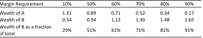
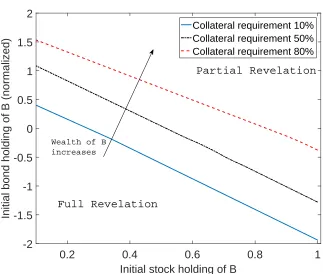
The model is then calculated according to the procedure outlined in the previous section to obtain a stationary equilibrium. Revelation depends on the wealth distribution at the beginning of each period. Since investor B needs to hold all stock in order for non-revelation to occur, the higher investor B's wealth, the more likely that non-revelation will happen. In Table 2, I show the equilibrium wealth cuto above which the signal of investor A is not revealed in state LL. When the margin requirement is 10%, non-revelation happens when investor B's equilibrium wealth is above 29% of the total wealth in the economy. It should be noted that since wealth depends on the equilibrium prices, the cuto given in Table 2 is also a quantity that is determined in equilibrium. The wealth distribution of investors is changing over time in a dynamic setting so we would see investor A go in and out of the stock market, which is accompanied by partial revelation.
If we tighten the collateral constraint in the economy, less borrowing is allowed. This would impede the ability of investor B to hold all of the stock through borrowing. Alter-natively, investor A cannot save all of her non consumed wealth in bonds because investor B cannot absorb all of the borrowing due to the tighter borrowing constraint. For either interpretation, partial revelation happens only when investor B has higher wealth at the beginning of a period. As can be seen in Table 2, the wealth cuto increases from 29% to 15It can be shown that when both agents have the same discount factor, the stock price is uniquely solved
91% as the collateral constraint moves from 10% to 90%. Figure 4 shows a similar message. The plot shows the regions of full and partial revelation given the wealth of investor B in equilibrium. Each line in the plot separates the full revelation and partial revelation regions for the corresponding level of collateral requirement. As the collateral constraint gets tighter, the region of fully revelation expands as the initial wealth requirement is higher for investor B in order to have partial revelation.
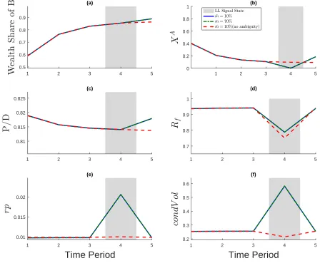
In order to see how the dynamics of the wealth distribution can aect revelation, I conduct two numerical experiments based on the stationary distribution. Both experiments last for ve periods and start with investor A holding 40% of the stock and no bonds. The realized signals in all periods are HH, but in period 4, the signal is LL in both experiments. In this case, partial revelation is only possible in period 4. The two experiments dier in the realizations of dividend growth. In experiment 1, the dividend grows at 13% per period, which corresponds to the value for H in Table 1. In experiment 2, the dividend declines 40%
per period. This dierence in dividend growth would result in dierent wealth distribution dynamics. Since investor B is less ambiguity and more patient than investor A, investor B holds more stock than investor A on average. A sequence of high dividend growth would lead to an increase in the relative wealth of investor B. This is shown in panel (a) of Figure 5. I simulated three series for each experiment: an unconstrained case (10% collateral requirement), a constrained case (70% collateral requirement), and a no-ambiguity case (10% collateral requirement without ambiguity aversion). Panel (a) shows that the wealth fraction of investor B grows from 60% to about 85% in period 3 for all three series. The shaded area in period 5 indicates the LL signal state. Panel (b) shows investor A's holdings of stock at the end of each period. Investor A holds a strictly positive amount of stock for all periods for the no-ambiguity case. For both cases of ambiguity, investor A exits the stock market in period 5 when the bad signal LL hits, resulting in partial revelation. We can see that the reduction in A's stock holdings also aects the wealth distribution for period 5 after the bad signal in period 4. The wealth fraction of B increases more in the two cases with ambiguity relative to the case without ambiguity, since investor A holds no or less stock in period 4 under ambiguity, leading the wealth to diverge when good dividend growth hits in period 5. The increase in the price dividend ratio (P=D) in period 5 amplies the divergence.
The risk-free rate (rf) drop in period 5 across all three series due to the bad signal
and HL. The conditional risk premium is computed as rpt = Et((Pt+1+ Dt+1)=PtRt). The
conditional risk premium is higher for the two cases with ambiguity since a higher premium is required for investor B to hold more risky assets than she would under no ambiguity. The conditional risk premium is higher for the constrained case because the interest rate is lower, as mentioned before. The conditional volatility of the stock return is computed as condV olt = fV art[(Pt+1+ Dt+1)=Pt]g1=2. The conditional volatility of the stock return rises
in the period with partial revelation. This is because the equilibrium price incorporates less information due to partial revelation and becomes a less accurate prediction for the payo of the stock next period.
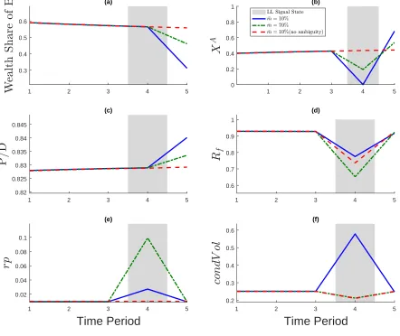
In the experiment with a sequence of low dividend growth, the wealth share of investor B declines slightly over time as in Figure 6. When the bad signal LL arrives in period 4, the wealth fraction of investor B can fall below the wealth cuto needed for partial revelation. For the unconstrained case, investor A still exits in period 4 when the LL signal is realized. However, the the constrained case, investor A reduces her stock holdings in period 4 but does not leave the market completely as seen in panel (b) of Figure 6. The conditional risk premium rises in period 4 for both cases with ambiguity, with the premium being highest in the constrained case. The conditional volatility of the stock return, on the other hand, is not higher in the constrained cases with ambiguity relative to the benchmark. This is because the equilibrium is fully revealing and prices incorporate all of the information that investors have.
To show the time-series properties of the model, I simulate time series for 3,000 periods and compute the moments of various variables. Table 3 summarizes the ndings. Panel (a) shows the unconstrained case when the collateral requirement is 10%, while panel (b) shows the case when the collateral requirement could be binding in some periods. For each variable, I show the mean, the standard deviation, and the rst-order auto correlation coecient (acf). The price dividend ratio and interest rate are slightly under ambiguity relative to the benchmark without ambiguity for both the unconstrained and constrained cases. The numerical dierences are small, though, due to the iid shocks of the model. High or low dividend growth matters little when the shock is not persistent relative to the investors' innite lifespan. The models with ambiguity can generate a higher and more volatile conditional risk premium. This is particularly true for the unconstrained case, as we saw in the simulations in the previous section. ip is an indicator variable that takes value
41% of periods are partially revealed in the unconstrained case. This percentage drops to about 5% when the collateral constraint is tighter.
4. Welfare Comparison
The analysis in the previous sections suggests that one policy instrument, collateral con-straints, could be used to help the market reveal information. In this section, I compute the welfare of the two investors for dierent levels of collateral constraints. The parameters used for the calculation in this section are the same as in Table 1. Figure 7 reports the expected welfare under the stationary distribution for both investors. The numbers are normalized to 1 for the case with a 10% collateral constraint. As we tighten the collateral constraint from 10% to 90%, the welfare of the investors does not move in a monotonic fashion. A tighter collateral requirement could lead to a Pareto improvement. For example, the welfare of both investors is higher at an 60% collateral constraint than at the 10% level.
A tighter collateral constraint generally has an ambiguous eect on welfare. This is because tighter collateral constraints aect welfare through two channels. As seen in the previous section, a tighter collateral requirement makes the market more transparent by reducing exits of investor A. This improves the information content of prices and lowers volatility in asset returns. However, a tighter collateral requirement also aects uncertainty sharing. Investors cannot share uncertainty as well when the collateral requirement is tighter, which decreases eciency. Hence, the overall eect of the collateral requirement on welfare is ambiguous.
5. Empirical Evidence
In this section, I investigate the empirical evidence against the ndings of the model. The model suggests that prices are less informative when investors exit and when there is higher concentration of ownership of a stock. Specically, I attempt to check whether a price informativeness measure of stocks respond to the extensive margin changes in investment by institutional investors.
investor has private information that is not perfectly correlated with each other. The exit of an institutional investor of a stock could lead to her private information not fully revealed in the price. Since her private information is not perfectly correlated with that of the other investors, some information is lost when she exits. Hence, we would expect the price of a stock becomes less informative when more investors exit the stock.
Second, there is only one stock in the model, but there are many stocks in the data. This will not be a problem if investors have private information of the idiosyncratic returns of stocks and the idiosyncratic returns of stocks are orthogonal to each other. To see this point, consider the CAPM model, where the return of a stock can be decomposed into two components: the systemic component and the idiosyncratic component. By denition, the idiosyncratic components of stock returns are independent of each other. If investors have private information about the idiosyncratic returns, then an investor's private information would not be fully revealed regardless of her trading action of other stocks. The partial-revelation result of the model survives even in a market with more than one stock. So the empirical analysis based on a panel of stock returns and institutional investors will be useful to study the theoretical ndings of the paper.
5.1. Data
To get a measure of extensive margin changes in investment of stocks, I obtain information on institutional stock holdings. Institutions with assets under management of over $100 million are required to le form 13F every quarter to the SEC. The ling information includes the amount of stocks held the end of each quarter. This gives us a snapshot of institutional investors' stock positions each quarter. Institutional investors include hedge funds, banks, insurance companies, mutual funds, pension funds, and endowment foundations. This group of investors maps naturally to the traders in the model. Institutional investors account for most market activity and frequently enter and exit individual stocks. They also do market research to gather information and then choose optimal portfolios. The stock-holding data are at the parent-rm level.
Since the 13F data contains all the institutional owners of a stock, we can count the number of institutional investors holding each stock for each quarter. Let Ni;t be the number
investors for a stock i. The main data set is then created through merging the 13F and CRSP data by CUSIP at the stock level. The sample period is from 1980 Q2 to 2011 Q4. The unit of observation of the data set is a stock-quarter pair.
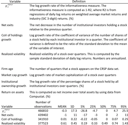
I obtain Data on stock returns and prices from CRSP at a daily frequency for US stocks to construct a price informativeness measure as in Chen et al. (2007). The price informativeness measure for stock i in quarter t is constructed as INF Oit = 1 R2it, where the R2itis estimated
through the regression of daily rm returns on market and industry returns given by
rijd= i0+ imrmd+ ijrjd+ "id:
rijd is the log returns of the stock of rm i in industry j on day d. rmd is the value weighted
log market return. And rjd is the value weighted log industry returns at the SIC 3-digit
level. R2
it is obtained from running the regression on daily data for each stock i and for each
quarter t. Then the informativeness measure IF NOit is computed for each stock for every
quarter as 1 R2
it. The idea is that high variation of idiosyncratic changes in prices are
correlated with more private information. In other words, stock prices contain less private information if the returns are mostly following market and industry returns, as reected by a high R2
it. The mean of INF Oit in the sample is 0.89 with a standard deviation of 0.14. The
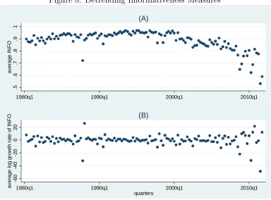
numbers are similar to those that are reported in Roll (1988) and Chen et al. (2007). The INF Oit exhibits some overall trend, with a moderate decline after 2000. Since the model
implication is on the time-series dimension, I detrend the series by focusing on the growth rate of INF Oit to avoid spurious regression results.16 The change in price informativeness
is dened to be the log growth rate of INF Oit over time, gitINF O = log(INF Oit=INF Oit 1).
To measure the degree of unequal holdings of shares of stock among institutional investors, I compute the coecient of variance of holdings CoVit = mean(sharesikt)=sd(sharesikt),
where sharesikt is the number of shares of stock i held by institutional investor k in quarter
t. The mean and standard deviation are taken over institutional investors for each stock i and quarter t. CoVit is higher when stock holdings are less equal. If all investors hold the
same amount of shares of a stock, the coecient of variance is zero. In the regression, the log growth rate of CoVit is used to eliminate the trend.
Other control variables, including realized volatility, rm age, market capitalization, and return on assets are dened in Table 4. Log growth rates of some variables are used to detrend the series in order to avoid spurious regression results. Summary statistics of all 16Appendix D plots the average of INF Oitfor each quarter across stocks and that of the log growth rate
variables are also shown in the lower panel of Table 4. Since I am interested in testing the time-series implication of the model, I restrict the sample to stocks that have at least 40 quarters of observations. Stocks in the nancial industries (SIC code 6000-6999) are also excluded from the sample.
5.2. Results
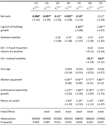
To see whether exits of investors lead to reduced informativeness of price of a stock, I run a regression of informativeness growth gINF O
it on net exits of investors ni;t. Column 1 in
Table 5 shows that more exits of investors are associated with lower informativeness. For example, a one standard deviation increase in the number of exits (about 11) is associated with about 0.1 percentage point lower growth rate of the informativeness measure. This is a 33% reduction from the mean growth rate. Similar result is reported in column 2 when stock xed eects are included in the regression to control for time invariant stock characteristics. To control for the underlying increase in volatility, realized return volatility is included in the regression in column 3. The coecient estimate of the realized volatility is negative, indicating higher volatility may lead to less informative prices, but the estimate is not statistically signicant. The coecient estimate of net exits remain signicant and its magnitude becomes larger. Regression in column 4 includes more control variables like rm age, market cap growth rate, institutional ownership growth and return on assets. The result that net exits is negatively associated with the informativeness remains the same. This is exactly what the model implies.
The model suggests that more unequal holding of the stock at the beginning of a period can lead to less information being revealed. In column 5 of Table 5, the lagged growth rate of the coecient of variance growth of share holdings is included in the regression. A lag value of the variable is consistent with the timing of the model. The result indeed conrms that growing dispersion of share holdings is associated with lower informativeness. A one standard deviation increase (0.22) in the lagged CoV is related to a 0.26 percentage point decrease in information growth. The regression results are consistent with what the model implies.
the last 4 quarters and zero otherwise.17 Then regressions are run on realized volatility, the
dummy variable, and the interaction term of the two in addition to the control variables. The coecient for the interaction term should be positive if volatility (a measure of underlying uncertainty) has a stronger eect on information loss after four consecutive periods of positive returns. Column 7 of the table shows that this is true in the data. If volatility is 10 percentage points higher after four quarters of positive returns, the informativeness measure growth rate is about 1 percentage points lower. However, if volatility is higher but not after a boom period (Dit = 0), the coecient is not statistically signicant. Column 8 shows similar results when
net exits and lag CoV are included in the regression.
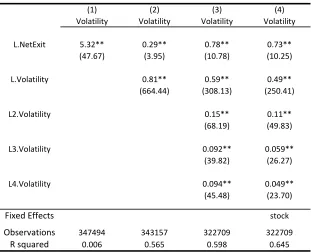
One implication in the model is that exits of investors predict higher future return volatil-ity. When the less ambiguous investor exits the market, the conditional future volatility of returns is higher due to less information being incorporated in prices. Hence, I would like to see whether higher exit rates of a stock are correlated with higher future stock return volatility. Table 6 shows the results of regressions of quarterly realized volatility on lagged net exit rates. The realized volatility is computed as the the standard deviation of daily log stock returns over a quarter. The numbers are then annualized and are in percentage. The coecient in column (1) of the table suggests that a higher exit rate predicts higher realized volatility next quarter. Volatility is well known to be serially correlated. The signicant co-ecient estimate may be a result of the concurrent correlation between volatility and exits, rather than of predictability. To control for the serial correlation of volatility, column (2) controls for the lagged value of volatility. It is not surprising to see that the coecient esti-mate of lagged net exit decreases by a lot, but it remains signicant. A 11 percentage point increase (about one standard deviation) in the next exit rate leads to the return volatility that is 2.9 percentage points higher in annual term. column (3) adds more lagged values of volatility to the regression. The coecient estimate of lagged net exit actually becomes bigger and more signicant. Finally, column (4) includes the stock xed eects to account for time invariant stock characteristics that might aect the level of volatility. The coecient of interest changes very little. Overall, we do see evidence that more exits of investors are associated with higher future return volatility.
17The results are not sensitive to the choice of the length of boom. Similar results are found with a dierent
6. Conclusion
This paper provides a useful framework to study endogenous market participation and in-formation aggregation. The model in this paper generates endogenous co-movement of non participation, conditional risk premia, and information eciency. In addition, it demon-strates the important roles of the wealth distribution and collateral requirements in informa-tion aggregainforma-tion. Empirical evidence supports that exits of investors move negatively with informativeness of prices.
A couple of extensions can be incorporated using the framework of the model in this paper. The model could use more persistent dividend growth shocks rather than the iid structure it currently has. Persistent dividend growth will lead to amplied eects that are not examined in the paper, since lower dividend growth or a bad signal means not just lower dividend growth in the next period, but for many periods to come. The increases the chance that the more ambiguity-averse investor stays out of the market for a longer period of time, which leads to more persistence in information loss.
References
Abel, A. B. (1990). Asset Prices Under Heterogenous Beliefs: Implications for the Equity Premium. Rodney L. White Center for Financial Research Working Papers 09-89, Wharton School Rodney L. White Center for Financial Research.
Admati, A. R. (1985). A Noisy Rational Expectations Equilibrium for Multi-asset Securities Markets. Econometrica, 53(3):62957.
Ahn, D., Choi, S., Gale, D., and Kariv, S. (2007). Estimating Ambiguity Aversion in a Portfolio Choice Experiment. Levine's working paper archive, David K. Levine.
Ahn, S., Choi, K. J., and Koo, H. K. (2015). A simple asset pricing model with heteroge-neous agents, uninsurable labor income and limited stock market participation. Journal of Banking & Finance, 55(C):922.
Allen, B. (1981). Generic Existence of Completely Revealing Equilibria for Economies with Uncertainty When Prices Convey Information. Econometrica, 49(5):11731199.
Allen, B. and Jordan, J. S. (1998). The Existence of Rational Expectations Equilibrium: A Retrospective. Sta Report 252, Federal Reserve Bank of Minneapolis.
Atmaz, A. and Basak, S. (2016). Belief dispersion in the stock market. SSRN Working Paper.
Banerjee, S. and Kremer, I. (2010). Disagreement and learning: Dynamic patterns of trade. The Journal of Finance, 65(4):12691302.
Basak, S. (2000). A model of dynamic equilibrium asset pricing with heterogeneous beliefs and extraneous risk. Journal of Economic Dynamics and Control, 24(1):63 95.
Basak, S. (2005). Asset pricing with heterogeneous beliefs. Journal of Banking & Finance, 29(11):2849 2881. Thirty Years of Continuous-Time Finance.
Bhamra, H. S. and Uppal, R. (2014). Asset prices with heterogeneity in preferences and beliefs. The Review of Financial Studies, 27(2):519.