v
Ba
BDescribing Motion:
Kinematics in One Dimension
2
C
H
A
P
T
E
R
The space shuttle has released a parachute to reduce its speed quickly. The directions of the shuttle’s velocity and acceleration are shown by the green and gold arrows.Motion is described using the concepts of velocity and acceleration. In the case shown here, the velocity is to the right, in the direction of motion. The acceleration is in the opposite direction from the velocity which means the object is slowing down.
We examine in detail motion with constant acceleration, including the vertical motion of objects falling under gravity.
v
B,
aB
v
B AaBB AvBB
21
CONTENTS2–1 Reference Frames and Displacement 2–2 Average Velocity 2–3 Instantaneous Velocity 2–4 Acceleration
2–5 Motion at Constant Acceleration 2–6 Solving Problems 2–7 Freely Falling Objects 2–8 Graphical Analysis of
Linear Motion CHAPTER-OPENING QUESTION—Guess now!
[Don’t worry about getting the right answer now—youwill get another chance later in the Chapter. See also p. 1 of Chapter 1 for more explanation.]
Two small heavy balls have the same diameter but one weighs twice as much as the other. The balls are dropped from a second-story balcony at the exact same time. The time to reach the ground below will be:
(a) twice as long for the lighter ball as for the heavier one. (b) longer for the lighter ball, but not twice as long. (c) twice as long for the heavier ball as for the lighter one. (d) longer for the heavier ball, but not twice as long. (e) nearly the same for both balls.
T
he motion of objects—baseballs, automobiles, joggers, and even the Sun and Moon—is an obvious part of everyday life. It was not until the sixteenth and seventeenth centuries that our modern understanding of motion was established. Many individuals contributed to this understanding, particularly Galileo Galilei (1564–1642) and Isaac Newton (1642–1727).22
CHAPTER 2 Describing Motion: Kinematics in One DimensionFIGURE 2;2 A person walks toward the front of a train at The train is moving with respect to the ground, so the walking person’s speed, relative to the ground, is 85 km兾h.
80 km兾h
5 km兾h.
For now we only discuss objects that move without rotating (Fig. 2–1a). Such motion is called translational motion. In this Chapter we will be concerned with describing an object that moves along a straight-line path, which is one-dimensional translational motion. In Chapter 3 we will describe translational motion in two (or three) dimensions along paths that are not straight. (Rotation, shown in Fig. 2–1b, is discussed in Chapter 8.)
We will often use the concept, or model, of an idealized particle which is considered to be a mathematical pointwith no spatial extent (no size). A point particle can undergo only translational motion. The particle model is useful in many real situations where we are interested only in translational motion and the object’s size is not significant. For example, we might consider a billiard ball, or even a spacecraft traveling toward the Moon, as a particle for many purposes.
2–1
Reference Frames and Displacement
Any measurement of position, distance, or speed must be made with respect to a reference frame, or frame of reference. For example, while you are on a train traveling at suppose a person walks past you toward the front of the train at a speed of, say, (Fig. 2–2). This is the person’s speed with respect to the train as frame of reference. With respect to the ground, that person is moving at a speed of It is always important to specify the frame of reference when stating a speed. In everyday life, we usually mean “with respect to the Earth” without even thinking about it, but the reference frame must be specified whenever there might be confusion.
80 km兾h + 5 km兾h = 85 km兾h. 5 km兾h
5 km兾h 80 km兾h,
(a) (b)
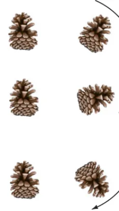
FIGURE 2;1 A falling pinecone undergoes (a) pure translation; (b) it is rotating as well as translating.
When specifying the motion of an object, it is important to specify not only the speed but also the direction of motion. Often we can specify a direction by using north, east, south, and west, and by “up” and “down.” In physics, we often draw a set of coordinate axes, as shown in Fig. 2–3, to represent a frame of reference. We can always place the origin 0, and the directions of the xand yaxes, as we like for convenience. The xand yaxes are always perpendicular to each other. The originis where Objects positioned to the right of the origin of coordinates (0) on the xaxis have an xcoordinate which we almost always choose to be positive; then points to the left of 0 have a negative xcoordinate. The position along the yaxis is usually considered positive when above 0, and negative when below 0, although the reverse convention can be used if convenient. Any point on the plane can be specified by giving its xandy coor-dinates. In three dimensions, a zaxis perpendicular to the xandyaxes is added. For one-dimensional motion, we often choose the xaxis as the line along which the motion takes place. Then the positionof an object at any moment is given by its xcoordinate. If the motion is vertical, as for a dropped object, we usually use the yaxis.
y = 0. x = 0,
− y + y
+ x − x
0
SECTION 2–2 Average Velocity
23
C A U T I O NThe displacement may not equal the total distance traveled
We need to make a distinction between the distancean object has traveled and its displacement, which is defined as the change in position of the object. That is, displacement is how far the object is from its starting point. To see the distinction between total distance and displacement, imagine a person walking 70 m to the east and then turning around and walking back (west) a distance of 30 m (see Fig. 2–4). The total distance traveled is 100 m, but the displacementis only 40 m since the person is now only 40 m from the starting point. Displacement is a quantity that has both magnitude and direction. Such quantities are called vectors, and are represented by arrows in diagrams. For example, in Fig. 2–4, the blue arrow represents the displacement whose magni-tude is 40 m and whose direction is to the right (east).
We will deal with vectors more fully in Chapter 3. For now, we deal only with motion in one dimension, along a line. In this case, vectors which point in one direc-tion will be positive (typically to the right along the xaxis). Vectors that point in the opposite direction will have a negative sign in front of their magnitude.
Consider the motion of an object over a particular time interval. Suppose that at some initial time, call it the object is on the xaxis at the position in the coordinate system shown in Fig. 2–5. At some later time, suppose the object has moved to position The displacement of our object is and is represented by the arrow pointing to the right in Fig. 2–5. It is convenient to write
where the symbol (Greek letter delta) means “change in.” Then means “the change in x,” or “change in position,” which is the displacement. The change in any quantity means the final value of that quantity, minus the initial value. Suppose and as in Fig. 2–5. Then
so the displacement is 20.0 m in the positive direction, Fig. 2–5.
Now consider an object moving to the left as shown in Fig. 2–6. Here the object, a person, starts at and walks to the left to the point
In this case her displacement is
and the blue arrow representing the vector displacement points to the left. For one-dimensional motion along the x axis, a vector pointing to the right is positive, whereas a vector pointing to the left has a negative sign.
EXERCISE A An ant starts at on a piece of graph paper and walks along the x axis to It then turns around and walks back to
Determine (a) the ant’s displacement and (b) the total distance traveled.
2–2
Average Velocity
An important aspect of the motion of a moving object is how fast it is moving—its speed or velocity.
The term “speed” refers to how far an object travels in a given time interval, regardless of direction. If a car travels 240 kilometers (km) in 3 hours (h), we say its average speed was In general, the average speed of an object is defined as the total distance traveled along its path divided by the time it takes to travel this distance:
(2;1)
The terms “velocity” and “speed” are often used interchangeably in ordi-nary language. But in physics we make a distinction between the two. Speed is simply a positive number, with units. Velocity, on the other hand, is used to signify both the magnitude (numerical value) of how fast an object is moving and also the direction in which it is moving. Velocity is therefore a vector.
average speed = distance traveled time elapsed . 80 km兾h.
x = –10cm. x = –20cm.
x= 20cm
¢x = x2 - x1 = 10.0 m - 30.0 m = –20.0 m,
x2 = 10.0 m. x1 =
30.0 m
¢x = x2 - x1 = 30.0 m - 10.0 m = 20.0 m, x2 = 30.0 m,
x1 = 10.0 m
¢x
¢
¢x = x2 - x1,
x2 - x1, x2.
t2,
x1 t1,
y
x
x2 x1
10 0
20 30 40 Distance (m)
x
x 0
70 m
West 40 m East
Displacement 30 m y
FIGURE 2;4 A person walks 70 m east, then 30 m west. The total distance traveled is 100 m (path is shown dashed in black); but the displacement, shown as a solid blue arrow, is 40 m to the east.
x y
x1 x2
10 0
20 30 40 Distance (m)
FIGURE 2;5 The arrow represents the displacement
Distances are in meters. x2 - x1.
FIGURE 2;6 For the displacement
the displacement vector points left.
There is a second difference between speed and velocity: namely, the average velocityis defined in terms of displacement, rather than total distance traveled:
Average speed and average velocity have the same magnitude when the motion is all in one direction. In other cases, they may differ: recall the walk we described earlier, in Fig. 2–4, where a person walked 70 m east and then 30 m west. The total distance traveled was but the displacement was 40 m. Suppose this walk took 70 s to complete. Then the average speed was:
The magnitude of the average velocity, on the other hand, was:
To discuss one-dimensional motion of an object in general, suppose that at some moment in time, call it the object is on the xaxis at position in a coordinate system, and at some later time, suppose it is at position The
elapsed time( in time) is during this time interval the
displacement of our object is Then the average velocity, defined as the displacement divided by the elapsed time, can be written
[average velocity] (2;2)
where stands for velocity and the bar over the is a standard symbol meaning “average.”
For one-dimensional motion in the usual case of the axis to the right, note that if is less than the object is moving to the left, and then is less than zero. The sign of the displacement, and thus of the average velocity, indicates the direction: the average velocity is positive for an object moving to the right along the axis and negative when the object moves to the left. The direction of the average velocity is always the same as the direction of the displacement.
It is always important to choose (and state) the elapsed time, or time interval, the time that passes during our chosen period of observation.
Runner’s average velocity. The position of a runner as a
function of time is plotted as moving along the xaxis of a coordinate system. During a 3.00-s time interval, the runner’s position changes from
to as shown in Fig. 2–7. What is the runner’s average velocity? APPROACH We want to find the average velocity, which is the displacement divided by the elapsed time.
SOLUTION The displacement is
The elapsed time, or time interval, is given as The average velocity (Eq. 2–2) is
The displacement and average velocity are negative, which tells us that the runner is moving to the left along the xaxis, as indicated by the arrow in Fig. 2–7. The runner’s average velocity is 6.50 m兾sto the left.
v = ¢x
¢t = – 19.5m
3.00s = –6.50 m兾s.
¢t = 3.00 s. = 30.5m -50.0m = –19.5m.
¢x = x2 -x1 x2 = 30.5m,
x1 = 50.0m
EXAMPLE 2;1
t2 - t1,
x
¢x = x2 - x1
x1,
x2 ±x
v ( )
v
v = x2t - x1 2 - t1
= ¢¢xt,
¢x = x2 - x1.
¢t = t2 - t1;
= change
x2. t2,
x1 t1,
displacement time elapsed =
40m
70s = 0.57 m兾s. distance
time elapsed = 100m
70s = 1.4 m兾s. 70m + 30m = 100m, average velocity = displacement
time elapsed =
final position - initial position time elapsed
.
24
CHAPTER 2 Describing Motion: Kinematics in One DimensionP R O B L E M S O L V I N G or sign can signify the direction
for linear motion ––
+ +
C A U T I O N
Average speed is not necessarily equal to the magnitude of the averagevelocity
y
x 10
0 20 30 40 50 60
Distance (m) Start
(x1) Finish
(x2)
x FIGURE 2;7 Example 2–1. A person runs from
to The displacement is–19.5m.
x2 = 30.5m.
x1 = 50.0m C A U T I O N
SECTION 2–3
25
Distance a cyclist travels. How far can a cyclist travel in
2.5 h along a straight road if her average velocity is
APPROACH We want to find the distance traveled, so we solve Eq. 2–2 for
SOLUTION In Eq. 2–2, we multiply both sides by and obtain
¢x = v¢t = (18 km兾h)(2.5 h) = 45 km.
¢t
v = ¢x兾¢t,
¢x. 18 km兾h?
EXAMPLE 2;2
FIGURE 2;8 Car speedometer showing in white, and in orange.
km兾h mi兾h
60
20 40
Velo
c
ity (k
m
/h)
Time (h)
(a)
0.2 0
Time (h)
(b)
0.5 0.1 0.3 0.4
0.2
0 0.1 0.3 0.4 0.5
Average velocity 0
60
20 40
Velo
c
ity (k
m
/h)
0
FIGURE 2;9 Velocity of a car as a function of time: (a) at constant velocity; (b) with velocity varying in time.
Car changes speed. A car travels at a constant for
100 km. It then speeds up to and is driven another 100 km. What is the car’s average speed for the 200-km trip?
APPROACH At the car takes 2.0 h to travel 100 km. At it
takes only 1.0 h to travel 100 km. We use the defintion of average velocity, Eq. 2–2. SOLUTION Average velocity (Eq. 2–2) is
NOTE Averaging the two speeds, gives
a wrong answer. Can you see why? You must use the definition of v, Eq. 2–2. 75 km兾h, (50 km兾h + 100 km兾h)兾2 =
v = ¢¢xt = 100km + 100km
2.0h + 1.0h = 67km兾h.
100 km兾h 50 km兾h,
100 km兾h
50 km兾h
EXAMPLE 2;3
2–3
Instantaneous Velocity
If you drive a car along a straight road for 150 km in 2.0 h, the magnitude of your average velocity is It is unlikely, though, that you were moving at precisely at every instant. To describe this situation we need the concept of instantaneousvelocity, which is the velocity at any instant of time. (Its magnitude is the number, with units, indicated by a speedometer, Fig. 2–8.) More precisely, the instantaneous velocity at any moment is defined as the averagevelocity over an infinitesimally short time interval. That is, Eq. 2–2 is to be evaluated in the limit of becoming extremely small, approaching zero. We can write the definition of instantaneous velocity, for one-dimensional motion as
[instantaneous velocity] (2;3)
The notation means the ratio is to be evaluated in the limit of approaching zero.†
For instantaneous velocity we use the symbol whereas for average velocity we use with a bar above. In the rest of this book, when we use the term “velocity” it will refer to instantaneous velocity. When we want to speak of the average velocity, we will make this clear by including the word “average.”
Note that the instantaneous speed always equals the magnitude of the instantaneous velocity. Why? Because distance traveled and the magnitude of the displacement become the same when they become infinitesimally small.
If an object moves at a uniform (that is, constant) velocity during a partic-ular time interval, then its instantaneous velocity at any instant is the same as its average velocity (see Fig. 2–9a). But in many situations this is not the case. For example, a car may start from rest, speed up to remain at that velocity for a time, then slow down to in a traffic jam, and finally stop at its destination after traveling a total of 15 km in 30 min. This trip is plotted on the graph of Fig. 2–9b. Also shown on the graph is the average velocity (dashed line), which is
Graphs are often useful for analysis of motion; we discuss additional insights graphs can provide as we go along, especially in Section 2–8.
v = ¢x兾¢t = 15km兾0.50h = 30km兾h. 20 km兾h
50 km兾h, v,
v,
¢t lim¢tS0 ¢x兾¢t v = lim
¢tS0
¢x
¢t.
v,
¢t 75km兾h
75km兾h.
†We do not simply set in this definition, for then would also be zero, and we would have
an undetermined number. Rather, we consider the ratio as a whole. As we let approach zero, approaches zero as well. But the ratio approaches some definite value, which is the instantaneous velocity at a given instant.
¢x兾¢t ¢x
¢t ¢x兾¢t,
¢x ¢t =0
26
CHAPTER 2 Describing Motion: Kinematics in One Dimension2–4
Acceleration
An object whose velocity is changing is said to be accelerating. For instance, a car whose velocity increases in magnitude from zero to is accelerating. Acceleration specifies how rapidlythe velocity of an object is changing.
Average acceleration is defined as the change in velocity divided by the time taken to make this change:
In symbols, the average acceleration, , over a time interval during which the velocity changes by is defined as
[average acceleration] (2;4)
We saw that velocity is a vector (it has magnitude and direction), so acceleration is a vector too. But for one dimensional motion, we need only use a plus or minus sign to indicate acceleration direction relative to a chosen coordinate axis. (Usually, right is left is .)
The instantaneous acceleration,a, can be defined in analogy to instantaneous velocity as the average acceleration over an infinitesimally short time interval at a given instant:
[instantaneous acceleration] (2;5)
Here ¢vis the very small change in velocity during the very short time interval ¢t. a = lim
¢tS0
¢v
¢t. – ±,
a = v2t - v1 2 - t1
= ¢¢vt.
¢v = v2 - v1,
¢t = t2 - t1, a
average acceleration = change of velocity time elapsed
. 80 km兾h
Acceleration
a = 15 km/hs
v1 = 0
t1 = 0
at t = 2.0 s
v = 30 km/h
at t = 1.0 s
v = 15 km/h
at t= t2 = 5.0 s
v=v2= 75 km/h
FIGURE 2;10 Example 2–4. The car is shown at the start with at The car is shown three more
times, at and at
the end of our time interval, The green arrows represent the velocity vectors, whose length represents the magnitude of the velocity at that moment. The acceleration vector is the orange arrow, whose magnitude is constant and equals or
(see top of next page). Distances are not to scale.
4.2m兾s2 15km兾h兾s
t2 = 5.0s. t= 2.0s,
t = 1.0s,
t1 = 0.
v1 = 0
Average acceleration. A car accelerates on a straight road from rest to in 5.0 s, Fig. 2–10. What is the magnitude of its average acceleration? APPROACH Average acceleration is the change in velocity divided by the elapsed time, 5.0 s. The car starts from rest, so The final velocity is . SOLUTION From Eq. 2–4, the average acceleration is
This is read as “fifteen kilometers per hour per second” and means that, on average, the velocity changed by 15 km h during each second. That is, assuming the acceleration was constant, during the first second the car’s velocity increased from zero to 15 km h. During the next second its velocity increased by another 15 km h, reaching a velocity of 30 km h at兾 兾 t = 2.0s, and so on. See Fig. 2–10.
兾
兾 a = v2 - v1
t2 - t1 =
75km兾h - 0km兾h
5.0s = 15
km兾h s .
v2 = 75 km兾h v1 = 0.
75 km兾h
SECTION 2–4 Acceleration
27
Our result in Example 2–4 contains two different time units: hours and seconds.We usually prefer to use only seconds. To do so we can change km h to m s (see Section 1–6, and Example 1–5):
Then
We almost always write the units for acceleration as (meters per second squared) instead of This is possible because:
Note that acceleration tells us how quickly the velocity changes, whereas velocity tells us howquickly the position changes.
m兾s s =
m ss =
m s2. m兾s兾s.
m兾s2 a = 21m兾s - 0.0m兾s
5.0s = 4.2 m兾s
s = 4.2 m s2. 75km兾h = a75 km
h b a 1000 m
1 km b a 1 h
3600 sb = 21m兾s.
兾 兾
Velocity and acceleration. (a) If the velocity of an object is zero, does it mean that the acceleration is zero? (b) If the acceleration is zero, does it mean that the velocity is zero? Think of some examples.
RESPONSE A zero velocity does not necessarily mean that the acceleration is zero, nor does a zero acceleration mean that the velocity is zero. (a) For example, when you put your foot on the gas pedal of your car which is at rest, the velocity starts from zero but the acceleration is not zero since the velocity of the car changes. (How else could your car start forward if its velocity weren’t changing—that is, accelerating?) (b) As you cruise along a straight highway at a constant velocity of 100 km兾h, your acceleration is zero: a = 0, v Z 0.
CONCEPTUAL EXAMPLE 2;5
C A U T I O N
Distinguishvelocity from acceleration
C A U T I O N
Ifvor a is zero, is the other zero too?
Acceleration
a= −2.0 m/s2
v1 = 15.0 m/s
at t1 = 0
v2 = 5.0 m/s
at t2 = 5.0 s
FIGURE 2;11 Example 2–6, showing the position of the car at times and as well as the car’s velocity represented by the green arrows. The acceleration vector (orange) points to the left because the car slows down as it moves to the right.
t2, t1
v1= −15.0 m/s
v2= −5.0 m/s
a
FIGURE 2;12 The car of
Example 2–6, now moving to the left and decelerating. The acceleration is
, or
= ±2.0m兾s2. = –5.0m兾s5.0+s15.0m兾s
a = (–5.0m兾s)5.0-(–s 15.0m兾s) a = (v2 - v1)兾¢t
Car slowing down. An automobile is moving to the right
along a straight highway, which we choose to be the positive xaxis (Fig. 2–11). Then the driver steps on the brakes. If the initial velocity (when the driver hits the brakes) is and it takes 5.0 s to slow down to
what was the car’s average acceleration?
APPROACH We put the given initial and final velocities, and the elapsed time, into Eq. 2–4 for
SOLUTION In Eq. 2–4, we call the initial time and set
The negative sign appears because the final velocity is less than the initial velocity. In this case the direction of the acceleration is to the left (in the negative x direc-tion)—even though the velocity is always pointing to the right. We say that the acceleration is 2.0m兾s2to the left, and it is shown in Fig. 2–11 as an orange arrow.
a = 5.0m兾s - 15.0m兾s
5.0s = –2.0 m兾s 2
.
t2 = 5.0s: t1 = 0,
a.
v2 = 5.0m兾s, v1 = 15.0m兾s,
EXAMPLE 2;6
Deceleration
When an object is slowing down, we can say it is decelerating. But be careful: deceleration does not mean that the acceleration is necessarily negative. The velocity of an object moving to the right along the positive xaxis is positive; if the object is slowing down (as in Fig. 2–11), the acceleration isnegative. But the same car moving to the left (decreasing x), and slowing down, has positive acceleration that points to the right, as shown in Fig. 2–12. We have a decelera-tion whenever the magnitude of the velocity is decreasing; thus the velocity and acceleration point in opposite directionswhen there is deceleration.
2–5
Motion at Constant Acceleration
We now examine motion in a straight line when the magnitude of the acceleration is constant. In this case, the instantaneous and average accelerations are equal. We use the definitions of average velocity and acceleration to derive a set of valuable equations that relate x, a, and when ais constant, allowing us to determine any one of these variables if we know the others. We can then solve many interesting Problems.
Notation in physics varies from book to book; and different instructors use different notation. We are now going to change our notation, to simplify it a bit for our discussion here of motion at constant acceleration. First we choose the initial time in any discussion to be zero, and we call it That is,
(This is effectively starting a stopwatch at ) We can then let be the elapsed time. The initial position and the initial velocity of an object will now be represented by and since they represent xand at At time the position and velocity will be called xand (rather than and ). The average velocity during the time interval will be (Eq. 2–2)
since we chose The acceleration, assumed constant in time, is (Eq. 2–4), so
A common problem is to determine the velocity of an object after any elapsed time when we are given the object’s constant acceleration. We can solve such problems†by solving for in the last equation: first we multiply both sides by ,
Then, adding to both sides, we obtain
[constant acceleration] (2;6)
If an object, such as a motorcycle (Fig. 2–13), starts from rest and accelerates at after an elapsed time its velocity will be
Next, let us see how to calculate the position xof an object after a time when it undergoes constant acceleration. The definition of average velocity (Eq. 2–2) is which we can rewrite by multiplying both sides by
(2;7)
Because the velocity increases at a uniform rate, the average velocity, will be midway between the initial and final velocities:
[constant acceleration] (2;8)
(Careful: Equation 2–8 is not necessarily valid if the acceleration is not constant.) We combine the last two Equations with Eq. 2–6 and find, starting with Eq. 2–7,
or
[constant acceleration] (2;9)
Equations 2–6, 2–8, and 2–9 are three of the four most useful equations for motion at constant acceleration. We now derive the fourth equation, which is useful
x = x0 + v0t + 1 2at2. = x0 + ¢v0 + v0 + at
2 ≤t
= x0 + ¢v0 + v
2 ≤t x = x0 + vt
v = v0 + v 2 .
v, x = x0 + vt.
t: v = Ax - x0B兾t,
t v = 0 + at = A4.0m兾s2B(6.0s) = 24m兾s. t =
6.0s
4.0m兾s2, Av0 =
0B v = v0 + at.
v0
at = v - v0 or v - v0 = at.
t v
t,
a = v -t v0.
a = ¢v兾¢t t0 = 0.
v = ¢x
¢t = xt -- x0t0
= x -t x0
t - t0
v2 x2 v
t x0 v0, v t = 0.
Av1B Ax1B t0. t2 = t
t1 = t0 = 0. t0.
t v,
28
CHAPTER 2C A U T I O N
Averagevelocity, but only if a = constant FIGURE 2;13 An accelerating motorcycle.
SECTION 2–5 Motion at Constant Acceleration
29
in situations where the time is not known. We substitute Eq. 2–8 into Eq. 2–7:Next we solve Eq. 2–6 for obtaining (see Appendix A–4 for a quick review)
and substituting this into the previous equation we have
We solve this for and obtain
[constant acceleration] (2;10)
which is the other useful equation we sought.
We now have four equations relating position, velocity, acceleration, and time, when the acceleration ais constant. We collect these kinematic equations for constant accelerationhere in one place for future reference (the tan background screen emphasizes their usefulness):
(2;11a) (2;11b) (2;11c)
(2;11d)
These useful equations are not valid unless ais a constant. In many cases we can set and this simplifies the above equations a bit. Note that x repre-sents position (not distance), also that is the displacement, and that is the elapsed time. Equations 2–11 are useful also when ais approximately constant to obtain reasonable estimates.
t x - x0
x0 = 0,
[a = constant] v = v + v0
2 .
[a = constant] v2 = v02 + 2aAx - x0B
[a = constant] x = x0 + v0t + 1
2at2
[a = constant] v = v0 + at
v2 = v02 + 2aAx - x0B, v2
x = x0 + ¢v + v0
2 ≤ ¢ v - v0
a ≤ = x0 + v 2 - v02
2a . t = v -av0,
t,
x = x0 + vt = x0 + ¢v + v0
2 ≤t. t
P R O B L E M S O L V I N G Equations 2–11 are valid only when the acceleration is constant,which we assume in this Example
P H Y S I C S A P P L I E D Airport design
Kinematic equations
for constant acceleration
(we’ll use them a lot)
Known Wanted
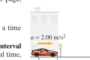
a = 2.00m兾s2 x = 150m v0 = 0
v x0 = 0
SOLUTION (a) Of the above four equations, Eq. 2–11c will give us when we know a, x, and
This runway length is notsufficient, because the minimum speed is not reached. (b) Now we want to find the minimum runway length, for a plane to reach given We again use Eq. 2–11c, but rewritten as
A 200-m runway is more appropriate for this plane.
NOTE We did this Example as if the plane were a particle, so we round off our answer to 200 m.
Ax - x0B = v 2 - v02
2a =
(27.8 m兾s)2 - 0
2A2.00m兾s2B = 193m. a = 2.00m兾s2.
v = 27.8m兾s,
x - x0, v = 3600m2兾s2 = 24.5m兾s.
= 0 + 2A2.00m兾s2B(150m) = 600m2兾s2 v2 = v02 + 2aAx - x0B
x0: v0,
v
Runway design. You are designing an airport for small
planes. One kind of airplane that might use this airfield must reach a speed before takeoff of at least and can accelerate at
(a) If the runway is 150 m long, can this airplane reach the required speed for takeoff? (b) If not, what minimum length must the runway have?
APPROACH Assuming the plane’s acceleration is constant, we use the kinematic equations for constant acceleration. In (a), we want to find and what we are given is shown in the Table in the margin.
v,
2.00 m兾s2. 27.8 m兾s(100 km兾h),
EXERCISE D A car starts from rest and accelerates at a constant during a -mile ( ) race. How fast is the car going at the finish line? (a)
(b) (c) (d)
2–6
Solving Problems
Before doing more worked-out Examples, let us look at how to approach problem solving. First, it is important to note that physics is nota collection of equations to be memorized. Simply searching for an equation that might work can lead you to a wrong result and will not help you understand physics (Fig. 2–14). A better approach is to use the following (rough) procedure, which we present as a special “Problem Solving Strategy.” (Other such Problem Solving Strategies will be found throughout the book.)
804 m兾s. 81 m兾s;
90 m兾s;
8040 m兾s; 402 m
1 4
10m兾s2
30
CHAPTER 2 Describing Motion: Kinematics in One Dimensionequation that involves only known quantities and one desired unknown, solve the equation alge-braically for the unknown. Sometimes several sequential calculations, or a combination of equa-tions, may be needed. It is often preferable to solve algebraically for the desired unknown before putting in numerical values.
7. Carry out the calculationif it is a numerical problem. Keep one or two extra digits during the calculations, but round off the final answer(s) to the correct number of significant figures (Section 1–4).
8. Think carefully about the result you obtain: Is it reasonable? Does it make sense according to your own intuition and experience? A good check is to do a rough estimate using only powers of 10, as discussed in Section 1–7. Often it is preferable to do a rough estimate at the start of a numerical problem because it can help you focus your attention on finding a path toward a solution. 9. A very important aspect of doing problems is
keep-ing track of units. An equals sign implies the units on each side must be the same, just as the numbers must. If the units do not balance, a mistake has been made. This can serve as a check on your solution (but it only tells you if you’re wrong, not if you’re right). Always use a consistent set of units.
P
R
O
B
L
E
M
S
O
LV I
N G
1. Read and rereadthe whole problem carefully before trying to solve it.
2. Decide what object (or objects) you are going to study, and for what time interval. You can often choose the initial time to be
3. Draw a diagram or picture of the situation, with coordinate axes wherever applicable. [You can place the origin of coordinates and the axes wherever you like to make your calculations easier. You also choose which direction is positive and which is negative. Usually we choose the xaxis to the right as positive.]
4. Write down what quantities are “known” or “given,” and then what you wantto know. Consider quan-tities both at the beginning and at the end of the chosen time interval. You may need to “translate” language into physical terms, such as “starts from rest” means
5. Think about which principles of physics apply in this problem. Use common sense and your own experiences. Then plan an approach.
6. Consider which equations(and/or definitions) relate the quantities involved. Before using them, be sure their range of validityincludes your problem (for example, Eqs. 2–11 are valid only when the accel-eration is constant). If you find an applicable
v0 = 0.
SECTION 2–6 Solving Problems
31
Acceleration of a car. How long does it take a car to cross
a 30.0-m-wide intersection after the light turns green, if the car accelerates from rest at a constant
APPROACH We follow the Problem Solving Strategy on the previous page, step by step.
SOLUTION
1. Rereadthe problem. Be sure you understand what it asks for (here, a time interval: “how long does it take”).
2. The object under study is the car. We need to choose the time interval during which we look at the car’s motion: we choose the initial time, to be the moment the car starts to accelerate from rest the time is the instant the car has traveled the full 30.0-m width of the intersection. 3. Drawadiagram: the situation is shown in Fig. 2–15, where the car is shown
moving along the positive xaxis. We choose at the front bumper of the car before it starts to move.
4. The “knowns” and the “wanted” information are shown in the Table in the margin. Note that “starting from rest” means at that is,
The wanted time is how long it takes the car to travel
5. The physics: the car, starting from rest at increases in speed as it covers more distance. The acceleration is constant, so we can use the kine-matic equations, Eqs. 2–11.
6. Equations: we want to find the time, given the distance and acceleration; Eq. 2–11b is perfect since the only unknown quantity is Setting
and in Eq. 2–11b we have
We solve for by multiplying both sides by :
Taking the square root, we get :
7. The calculation:
This is our answer. Note that the units come out correctly.
8. We can check the reasonablenessof the answer by doing an alternate calcu-lation: we first find the final velocity
and then find the distance traveled
which checks with our given distance.
9. We checked the unitsin step 7, and they came out correctly (seconds).
NOTE In steps 6 and 7, when we took the square root, we should have written Mathematically there are two solutions. But the second solution, is a time before our chosen time interval and makes no sense physically. We say it is “unphysical” and ignore it.
We explicitly followed the steps of the Problem Solving Strategy in Example 2–8. In upcoming Examples, we will use our usual “Approach” and “Solution” to avoid being wordy.
t = –5.48 s, t = &22x兾a = &5.48 s.
x = x0 + vt = 0 + 12(10.96m兾s + 0)(5.48s) = 30.0m, v = at = A2.00m兾s2B(5.48s) = 10.96m兾s,
t =
B
2x
a = C
2(30.0m)
2.00m兾s2 = 5.48 s. t =
B
2x a .
t 2x
a = t2.
2 a
t x = 1
2at2.
Ax = x0 + v0t + 1 2at2B, x0 = 0
v0 = 0 t.
t0 = 0B, A
30.0m.
t v = 0 t = 0; v0 = 0.
x0 = 0
t Av0 = 0B;
t = 0, 2.00m兾s2?
EXAMPLE 2;8
P R O B L E M S O L V I N G Check your answer
P R O B L E M S O L V I N G “Starting from rest” means
at t = 0 [i.e.,v0 = 0]
v = 0
Known Wanted
v0 = 0 a = 2.00m兾s2 x = 30.0m
t
x0 = 0
0
a= 2.00 m/s2 a= 2.00 m/s2
x0=0
v = 0 30.0 mx= FIGURE 2;15 Example 2–8.
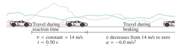
Braking distances. Estimate the minimum stopping distance for a car, which is important for traffic safety and traffic design. The problem is best dealt with in two parts, two separate time intervals. (1) The first time interval begins when the driver decides to hit the brakes, and ends when the foot touches the brake pedal. This is the “reaction time” during which the speed is constant, so (2) The second time interval is the actual braking period when the vehicle slows down and comes to a stop. The stopping distance depends on the reaction time of the driver, the initial speed of the car (the final speed is zero), and the deceleration of the car. For a dry road and good tires, good brakes can decelerate a car at a rate of about to
Calculate the total stopping distance for an initial velocity of and assume the acceleration of the car is
(the minus sign appears because the velocity is taken to be in the positive xdirection and its magnitude is decreasing). Reaction time for normal drivers varies from perhaps 0.3 s to about 1.0 s; take it to be 0.50 s.
APPROACH During the “reaction time,” part (1), the car moves at constant speed of so Once the brakes are applied, part (2), the acceler-ation is and is constant over this time interval. For both parts ais constant, so we can use Eqs. 2–11.
SOLUTION Part (1). We take for the first time interval, when the driver is reacting (0.50 s): the car travels at a constant speed of so
See Fig. 2–16 and the Table in the margin. To find x, the position of the car at (when the brakes are applied), we cannot use Eq. 2–11c because xis multiplied by a, which is zero. But Eq. 2–11b works:
Thus the car travels 7.0 m during the driver’s reaction time, until the instant the brakes are applied. We will use this result as input to part (2).
Part (2). During the second time interval, the brakes are applied and the car is brought to rest. The initial position is (result of part (1)), and other variables are shown in the second Table in the margin. Equation 2–11a doesn’t contain x; Eq. 2–11b contains x but also the unknown Equation 2–11c, is what we want; after setting we solve forx, the final position of the car (when it stops):
The car traveled 7.0 m while the driver was reacting and another 16 m during the braking period before coming to a stop, for a total distance traveled of 23 m. Figure 2–17 shows a graph of vs. is constant from until
and after it decreases linearly to zero.
NOTE From the equation above for x, we see that the stopping distance after the driver hit the brakes increases with the squareof the initial speed, not just linearly with speed. If you are traveling twice as fast, it takes four times the distance to stop.
A= x - x0B
t = 0.50 s t = 0.50 s,
t = 0 v
t: v
= 7.0 m + 16 m = 23 m. = 7.0m + 0 - (14 m兾s)
2
2A–6.0m兾s2B = 7.0m +
–196 m2兾s2 –12m兾s2 v2 - v02
2a
+
x = x0
x0 = 7.0m,
v2 - v02 = 2aAx - x0B, t
. x0 = 7.0m
x = v0t + 0 = (14 m兾s)(0.50 s) = 7.0 m. t = 0.50s
a = 0. 14 m兾s
x0 = 0 a = –6.0 m兾as2=
0. 14 m兾s,
–6.0m兾s2 (= 14m兾s L 31mi兾h)
50km兾h 8m兾s2.
5m兾s2 (a Z 0)
a = 0.
EXAMPLE 2;9 ESTIMATE
32
CHAPTER 2 Describing Motion: Kinematics in One DimensionP H Y S I C S A P P L I E D Car stopping distances
Travel during reaction time
Travel during braking = constant = 14 m/s
t = 0.50 s a = 0
a = −6.0 m/s2
x
decreases from 14 m/s to zero
v v
FIGURE 2;16 Example 2–9: stopping distance for a braking car.
Part 1: Reaction time
Known Wanted
x
x0 = 0 a= 0 v = 14m兾s v0 = 14m兾s t= 0.50s
Part 2: Braking
Known Wanted
x
a= –6.0m兾s2 v = 0
v0 = 14m兾s x0 = 7.0m
10 8 6
2 4 14 12
t (s)
v
(m/s)
t= 0.5 s
0 0.5 1.0 1.5 2.0 2.5
SECTION 2–7 Freely Falling Objects
33
2–7
Freely Falling Objects
One of the most common examples of uniformly accelerated motion is that of an object allowed to fall freely near the Earth’s surface. That a falling object is accelerating may not be obvious at first. And beware of thinking, as was widely believed before the time of Galileo (Fig. 2–18), that heavier objects fall faster than lighter objects and that the speed of fall is proportional to how heavy the object is. The speed of a falling object isnotproportional to its mass.
Galileo made use of his new technique of imagining what would happen in idealized (simplified) cases. For free fall, he postulated that all objects would fallwith the same constant acceleration in the absence of air or other resistance. He showed that this postulate predicts that for an object falling from rest, the distance traveled will be proportional to the square of the time (Fig. 2–19); that is, We can see this from Eq. 2–11b for constant acceleration; but Galileo was the first to derive this mathematical relation.
To support his claim that falling objects increase in speed as they fall, Galileo made use of a clever argument: a heavy stone dropped from a height of 2 m will drive a stake into the ground much further than will the same stone dropped from a height of only 0.2 m. Clearly, the stone must be moving faster in the former case.
Galileo claimed that all objects, light or heavy, fall with the same accel-eration, at least in the absence of air. If you hold a piece of paper flat and horizontal in one hand, and a heavier object like a baseball in the other, and release them at the same time as in Fig. 2–20a, the heavier object will reach the ground first. But if you repeat the experiment, this time crumpling the paper into a small wad, you will find (see Fig. 2–20b) that the two objects reach the floor at nearly the same time.
Galileo was sure that air acts as a resistance to very light objects that have a large surface area. But in many ordinary circumstances this air resistance is negligible. In a chamber from which the air has been removed, even light objects like a feather or a horizontally held piece of paper will fall with the same acceleration as any other object (see Fig. 2–21). Such a demonstration in vacuum was not possible in Galileo’s time, which makes Galileo’s achievement all the greater. Galileo is often called the “father of modern science,” not only for the content of his science (astronomical discoveries, inertia, free fall) but also for his new methods of doingscience (idealization and simplification, mathe-matization of theory, theories that have testable consequences, experiments to test theoretical predictions).
d r t2.
FIGURE 2;18 Painting of Galileo demonstrating to the Grand Duke of Tuscany his argument for the action of gravity being uniform acceleration. He used an inclined plane to slow down the action. A ball rolling down the plane still accelerates. Tiny bells placed at equal distances along the inclined plane would ring at shorter time intervals as the ball “fell,” indicating that the speed was increasing.
FIGURE 2;19 Multiflash photograph of a falling apple, at equal time intervals. The apple falls farther during each successive interval, which means it is accelerating.
(a) (b)
FIGURE 2;20 (a) A ball and a light piece of paper are dropped at the same time. (b) Repeated, with the paper wadded up.
Air-filled tube (a)
Evacuated tube (b) FIGURE 2;21 A rock and a feather are dropped simultaneously
Galileo’s specific contribution to our understanding of the motion of falling objects can be summarized as follows:
at a given location on the Earth and in the absence of air resistance, all objects fall with the same constant acceleration.
We call this acceleration the acceleration due to gravity at the surface of the Earth, and we give it the symbol g. Its magnitude is approximately
In British units gis about Actually, gvaries slightly according to lati-tude and elevation on the Earth’s surface, but these variations are so small that we will ignore them for most purposes. (Acceleration of gravity in space beyond the Earth’s surface is treated in Chapter 5.) The effects of air resistance are often small, and we will neglect them for the most part. However, air resistance will be noticeable even on a reasonably heavy object if the velocity becomes large.† Acceleration due to gravity is a vector, as is any acceleration, and its direction is downward toward the center of the Earth.
When dealing with freely falling objects we can make use of Eqs. 2–11, where for awe use the value of ggiven above. Also, since the motion is vertical we will substitute yin place of x, and in place of We take unless otherwise specified. It is arbitrary whether we choose y to be positive in the upward direction or in the downward direction; but we must be consistent about it throughout a problem’s solution.
EXERCISE E Return to the Chapter-Opening Question, page 21, and answer it again now, assuming minimal air resistance. Try to explain why you may have answered differently the first time.
Falling from a tower. Suppose that a ball is dropped
from a tower. How far will it have fallen after a time and Ignore air resistance.
APPROACH Let us take y as positive downward, so the acceleration is We set and We want to find the posi-tion y of the ball after three different time intervals. Equation 2–11b, with xreplaced by y, relates the given quantities ( a, and ) to the unknown y.
SOLUTION We set in Eq. 2–11b:
The ball has fallen a distance of 4.90 m during the time interval to Similarly, after 2.00 s the ball’s position is
Finally, after 3.00 s the ball’s position is (see Fig. 2–22)
NOTE Whenever we say “dropped,” it means Note also the graph of y vs. (Fig. 2–22b): the curve is not straight but bends upward because yis proportional to t2.
t v0 = 0.
y3 = 1 2at32 =
1
2A9.80m兾s
2B(3.00s)2 = 44.1m. A= t3B,
y2 = 1 2at22 =
1
2A9.80m兾s2B(2.00s)2 = 19.6m. A= t2B,
t1 = 1.00 s.
t = 0 = 0 + 12at2
1 = 1
2A9.80m兾s
2B(1.00s)2 = 4.90m. y1 = v0t1 +
1 2at
2 1 t = t1 = 1.00s
v0 t,
y0 = 0. v0 = 0
a = g = ±9.80 m兾s2. t3 = 3.00s? t2 = 2.00s,
t1 = 1.00s, (v0 = 0)
EXAMPLE 2;10
y0 = 0 x0.
y0 32 ft兾s2.
cacceleration due to gravityat surface of Earth d
g = 9.80 m兾s2.
P R O B L E M S O L V I N G You can choose y to be positive either up or down
†The speed of an object falling in air (or other fluid) does not increase indefinitely. If the object falls
far enough, it will reach a maximum velocity called the terminal velocitydue to air resistance.
34
CHAPTER 2 Describing Motion: Kinematics in One Dimension(a)
(b) 40 30 20 10
y
(m)
2
0 1 3
t(s)
y= 0
y3= 44.1 m (After 3.00 s)
y2= 19.6 m (After 2.00 s)
y1= 4.90 m (After 1.00 s)
+y Acceleration
due to gravity
+y
SECTION 2–7 Freely Falling Objects
35
Thrown down from a tower. Suppose the ball in
Example 2–10 is throwndownward with an initial velocity of instead of being dropped. (a) What then would be its position after 1.00 s and 2.00 s? (b) What would its speed be after 1.00 s and 2.00 s? Compare with the speeds of a dropped ball.
APPROACH Again we use Eq. 2–11b, but now is not zero, it is
SOLUTION (a) At the position of the ball as given by Eq. 2–11b is
At (time interval to ), the position is
As expected, the ball falls farther each second than if it were dropped with
(b) The velocity is obtained from Eq. 2–11a:
[at ] [at ]
In Example 2–10, when the ball was dropped the first term in these equations was zero, so
[at ] [at ]
NOTE For both Examples 2–10 and 2–11, the speed increases linearly in time by during each second. But the speed of the downwardly thrown ball at any instant is always (its initial speed) higher than that of a dropped ball.
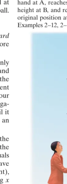
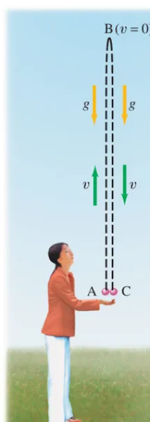
Ball thrown upward. A person throws a ball upward
into the air with an initial velocity of Calculate how high it goes. Ignore air resistance.
APPROACH We are not concerned here with the throwing action, but only with the motion of the ball after it leaves the thrower’s hand (Fig. 2–23) and until it comes back to the hand again. Let us choose y to be positive in the upward direction and negative in the downward direction. (This is a different convention from that used in Examples 2–10 and 2–11, and so illustrates our options.) The acceleration due to gravity is downward and so will have a nega-tive sign, As the ball rises, its speed decreases until it reaches the highest point (B in Fig. 2–23), where its speed is zero for an instant; then it descends, with increasing speed.
SOLUTION We consider the time interval from when the ball leaves the thrower’s hand until the ball reaches the highest point. To determine the maximum height, we calculate the position of the ball when its velocity equals zero ( at the highest point). At (point A in Fig. 2–23) we have
and At time (maximum height),
and we wish to find y. We use Eq. 2–11c, replacing x withy: We solve this equation for y:
The ball reaches a height of 11.5 m above the hand. y = v
2 - v02
2a =
0 - (15.0m兾s)2
2A–9.80m兾s2B = 11.5m. v2 = v02 +
2ay. a = –9.80 m兾s2, v = 0,
t a = –9.80 m兾s2.
v0 = 15.0 m兾s, y0 = 0,
t = 0 v = 0
a = –g = –9.80m兾s2.
15.0 m兾s.
EXAMPLE 2;12
3.00 m兾s 9.80 m兾s
t2 = 2.00s = A9.80m兾s2B(2.00s) = 19.6m兾s.
t1 = 1.00s = A9.80m兾s2B(1.00s) = 9.80m兾s
v = 0 + at
Av0B Av0 = 0B,
t2 = 2.00s = 3.00m兾s + A9.80m兾s2B(2.00s) = 22.6m兾s.
t1 = 1.00 s = 3.00 m兾s + A9.80 m兾s2B(1.00 s) = 12.8 m兾s
v = v0 + at v0 = 0.
y = v0t + 1
2at2 = (3.00m兾s)(2.00s) + 1
2A9.80m兾s2B(2.00s)2 = 25.6m. t = 2.00s
t = 0 t2 = 2.00s
y = v0t + 1
2at2 = (3.00m兾s)(1.00s) + 1
2A9.80m兾s2B(1.00s)2 = 7.90m. t1 = 1.00s,
v0 = 3.00 m兾s.
v0
3.00 m兾s,
EXAMPLE 2;11
A C
(v= 0) B
v v
g g
FIGURE 2;23 An object thrown into the air leaves the thrower’s hand at A, reaches its maximum height at B, and returns to the original position at C.
Ball thrown upward,II. In Fig. 2–23, Example 2–12, how long is the ball in the air before it comes back to the hand?
APPROACH We need to choose a time interval to calculate how long the ball is in the air before it returns to the hand. We could do this calculation in two parts by first determining the time required for the ball to reach its highest point, and then determining the time it takes to fall back down. However, it is simpler to consider the time interval for the entire motion from A to B to C (Fig. 2–23) in one step and use Eq. 2–11b. We can do this because yis position or displacement, and not the total distance traveled. Thus, at both points A and C,
SOLUTION We use Eq. 2–11b with and find
This equation can be factored (we factor out one ):
There are two solutions:
The first solution corresponds to the initial point (A) in Fig. 2–23, when the ball was first thrown from The second solution,
corresponds to point C, when the ball has returned to Thus the ball is in the air 3.06 s.
NOTE We have ignored air resistance in these last two Examples, which could be significant, so our result is only an approximation to a real, practical situation.
y = 0.
t = 3.06s, y = 0.
(t = 0)
t = 0 and t = 15.0 m兾s
4.90m兾s2 = 3.06s. A15.0m兾s - 4.90m兾s2tBt = 0.
t 0 = 0 + (15.0m兾s)t + 12A–9.80m兾s2Bt2. y = y0 + v0t + 1
2at2
a = –9.80m兾s2 y = 0.
EXAMPLE 2;13
36
CHAPTER 2 Describing Motion: Kinematics in One DimensionC A U T I O N
Quadratic equations have two solutions. Sometimes only one corresponds to reality, sometimes both
C A U T I O N
(1) Velocity and acceleration are not always in the same direction; the acceleration (of gravity) always points down (2) even at the highest point
of a trajectory a Z 0
Two possible misconceptions. Give
examples to show the error in these two common misconceptions: (1) that acceleration and velocity are always in the same direction, and (2) that an object thrown upward has zero acceleration at the highest point (B in Fig. 2–23).
RESPONSE Both are wrong. (1) Velocity and acceleration are notnecessarily in the same direction. When the ball in Fig. 2–23 is moving upward, its velocity is positive (upward), whereas the acceleration is negative (down-ward). (2) At the highest point (B in Fig. 2–23), the ball has zero velocity for an instant. Is the acceleration also zero at this point? No. The velocity near the top of the arc points upward, then becomes zero for an instant (zero time) at the highest point, and then points downward. Gravity does not stop acting, so even there. Thinking that at point B would lead to the conclusion that upon reaching point B, the ball would stay there: if the acceleration ( of change of velocity) were zero, the velocity would stay zero at the highest point, and the ball would stay up there without falling. Remember: the acceleration of gravity always points down toward the Earth, even when the object is moving up.
= rate
a = 0 a = –g = –9.80m兾s2
CONCEPTUAL EXAMPLE 2;14
We did not consider the throwing action in these Examples. Why? Because during the throw, the thrower’s hand is touching the ball and accelerating the ball at a rate unknown to us—the acceleration is not g. We consider only the time when the ball is in the air and the acceleration is equal to g.
Every quadratic equation (where the variable is squared) mathematically produces two solutions. In physics, sometimes only one solution corresponds to the real situation, as in Example 2–8, in which case we ignore the “unphysical” solution. But in Example 2–13, both solutions to our equation in are physi-cally meaningful: t = 0 and t = 3.06s.
t2
A C
(v= 0) B
v v
g g
FIGURE 2;23(Repeated.)
An object thrown into the air leaves the thrower’s hand at A, reaches its maximum height at B, and returns to the original position at C.
SECTION 2–7 Freely Falling Objects
37
Ball thrown upward,III. Let us consider again the ball
thrown upward of Examples 2–12 and 2–13, and make more calculations. Calculate (a) how much time it takes for the ball to reach the maximum height (point B in Fig. 2–23), and (b) the velocity of the ball when it returns to the thrower’s hand (point C).
APPROACH Again we assume the acceleration is constant, so we can use Eqs. 2–11. We have the maximum height of 11.5 m and initial speed of
from Example 2–12. Again we take yas positive upward.
SOLUTION (a) We consider the time interval between the throw
and the top of the path and we want to find The acceleration is constant at Both Eqs. 2–11a and 2–11b contain the time with other quantities known. Let us
use Eq. 2–11a with and
setting gives , which we rearrange to solve for : or
This is just half the time it takes the ball to go up and fall back to its original position [3.06 s, calculated in Example 2–13]. Thus it takes the same time to reach the maximum height as to fall back to the starting point.
(b) Now we consider the time interval from the throw
until the ball’s return to the hand, which occurs at (as calculated in Example 2–13), and we want to find when
NOTE The ball has the same speed (magnitude of velocity) when it returns to the starting point as it did initially, but in the opposite direction (this is the meaning of the negative sign). And, as we saw in part (a), the time is the same up as down. Thus the motion is symmetricalabout the maximum height.
= 15.0 m兾s - A9.80 m兾s2B(3.06 s) = –15.0 m兾s. v = v0 + at
t = 3.06 s:
v t = 3.06 s
At = 0, v0 = 15.0 m兾sB = – 15.0 m兾s
–9.80m兾s2 = 1.53s. t = – v0a
at = –v0 t
0 = v0 + at v = 0
v = v0 + at;
v = 0: a = –9.80m兾s2, v0t= 15.0m兾s,
a = –g = –9.80m兾s2. t.
(y = ±11.5m, v = 0), v0 = 15.0m兾sB
At = 0, 15.0 m兾s
EXAMPLE 2;15
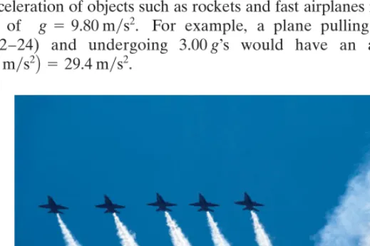
The acceleration of objects such as rockets and fast airplanes is often given as a multiple of For example, a plane pulling out of a dive (see Fig. 2–24) and undergoing 3.00g’s would have an acceleration of
. (3.00)A9.80m兾s2B = 29.4m兾s2
g = 9.80m兾s2.
P R O B L E M S O L V I N G Acceleration in g’s
38
CHAPTER 2 Describing Motion: Kinematics in One DimensionBall thrown upward at edge of cliff. Suppose that the
person of Examples 2–12, 2–13, and 2–15 throws the ball upward at while standing on the edge of a cliff, so that the ball can fall to the base of the cliff 50.0 m below, as shown in Fig. 2–25a. (a) How long does it take the ball to reach the base of the cliff? (b) What is the total distance trav-eled by the ball? Ignore air resistance (likely to be significant, so our result is an approximation).
APPROACH We again use Eq. 2–11b, with yas upward, but this time we set the bottom of the cliff, which is 50.0 m below the initial position hence the minus sign.
SOLUTION (a) We use Eq. 2–11b with and
To solve any quadratic equation of the form
wherea,b, and care constants (aisnotacceleration here), we use the quadratic formula(see Appendix A–4):
We rewrite our yequation just above in standard form,
Using the quadratic formula, we find as solutions
and
The first solution, is the answer we are seeking: the time it takes the ball to rise to its highest point and then fall to the base of the cliff. To rise and fall back to the top of the cliff took 3.06 s (Example 2–13); so it took an additional 2.01 s to fall to the base. But what is the meaning of the other solution, This is a time before the throw, when our calculation begins, so it isn’t relevant here. It is outside our chosen time interval, and so is anunphysicalsolution (also in Example 2–8).
(b) From Example 2–12, the ball moves up 11.5 m, falls 11.5 m back down to the top of the cliff, and then down another 50.0 m to the base of the cliff, for a total distance traveled of 73.0 m. [Note that the displacement, however, was
] Figure 2–25b shows the yvs. graph for this situation.t –50.0 m.
t = –2.01 s? t = 5.07 s, t = –2.01 s. t = 5.07 s
A4.90 m兾s2Bt2 - (15.0 m兾s)t - (50.0 m) = 0.
at2 + bt + c = 0: t = –b63b
2 - 4ac
2a .
at2 + bt + c = 0,
–50.0 m = 0 + (15.0 m兾s)t - 12A9.80 m兾s 2Bt2
. y = y0 + v0t + 1
2at 2 y = –50.0 m:
y0 = 0,
v0 = 15.0 m兾s, a = –9.80 m兾s2,
Ay0 = 0B; y = –50.0m,
+
15.0 m兾s
EXAMPLE 2;16
y
y=0
y=50 m
(a)
(b) 1
0 2 3 4 5 6
−40 −50 −30 −20 −10 0 10
t (s)
y
(m)
Base of cliff Hand
t= 5.07 s
FIGURE 2;25 Example 2–16. (a) A person stands on the edge of a cliff. A ball is thrown upward, then falls back down past the thrower to the base of the cliff, 50.0 m below. (b) The yvs. graph.t
Additional Example—Using the Quadratic Formula
EXERCISE F Two balls are thrown from a cliff. One is thrown directly up, the other directly down. Both balls have the same initial speed, and both hit the ground below the cliff but at different times. Which ball hits the ground at the greater speed: (a) the ball thrown upward, (b) the ball thrown downward, or (c) both the same? Ignore air resistance.
C A U T I O N
SECTION 2–8 Graphical Analysis of Linear Motion
39
2–8
Graphical Analysis of Linear Motion
Velocity as Slope
Analysis of motion using graphs can give us additional insight into kinematics. Let us draw a graph of xvs. making the choice that at the position of an object is and the object is moving at a constant velocity,
Our graph starts at (the origin). The graph of the position increases linearly in time because, by Eq. 2–2, and is a constant. So the graph of x vs. is a straight line, as shown in Fig. 2–26. The small (shaded) triangle on the graph indicates the slopeof the straight line:
We see, using the definition of average velocity (Eq. 2–2), that the slope of the xvs. graph is equal to the velocity. And, as can be seen from the small triangle
on the graph, which is the given velocity.
If the object’s velocity changes in time, we might have an xvs. graph like that shown in Fig. 2–27. (Note that this graph is different from showing the “path” of an object on an x vs. y plot.) Suppose the object is at position at time and at position at time and represent these two points on the graph. A straight line drawn from point to point
forms the hypotenuse of a right triangle whose sides are and The ratio is the slope of the straight line But is also the average velocity of the object during the time interval Therefore, we conclude that the average velocity of an object during any time interval is equal to the slope of the straight line(orchord) connecting the two points and on an xvs. graph.
Consider now a time intermediate between and call it at which moment the object is at (Fig. 2–28). The slope of the straight line is less than the slope of . Thus the average velocity during the time interval is less than during the time interval t2 - t1.
t3 - t1 P1P2
P1P3
x3 t3
, t2,
t1 t
t2B Ax2, t1B
Ax1,
¢t = t2 - t1
¢t = t2 - t1.
¢x兾¢t P1P2.
¢x兾¢t
¢t.
¢x
t2B P2Ax2, t1B
P1Ax1, P2 P1 t2. x2
t1,
x1 t
¢x兾¢t = (11m)兾(1.0s) = 11m兾s, t
slope = ¢x
¢t.
t ¢x = v¢t v
t = 0 x = 0, (40 km兾h).
v = v = 11 m兾s x = 0,
t = 0, t,
†The tangent is a straight line that touches the curve only at the one chosen point, without passing across or through the curve at that point.
Δ t= 1.0s
Δ x= 11 m 50
40
30
20
10
0
1.0 2.0 3.0 4.0 5.0 0
Position,
x
(m)
Time,t(s) FIGURE 2;26 Graph of position vs. time for an object moving at a constant velocity of 11m兾s.
P1
P2
Δx=x2−x1
Δt=t2−t1 t2 t1
x1 x2
0 x
t FIGURE 2;27 Graph of an object’s positionxvs. time . The slope of the straight line represents the average velocity of the object during the time interval ¢t = t2 - t1.
P1P2 t
P1
P2
t3
tangent at P 1
0 t1 t2
x1 x2
x
t P3
x3
x2 FIGURE 2;28 Same position vs. time curve
as in Fig. 2–27. Note that the average velocity over the time interval
(which is the slope of ) is less than the average velocity over the time interval
The slope of the line tangent to the curve at point equals the instantaneousvelocity at time t1.
P1 t2 - t1.
P1P3
t3 - t1
Next let us take point in Fig. 2–28 to be closer and closer to point That is, we let the interval which we now call to become smaller and smaller. The slope of the line connecting the two points becomes closer and closer to the slope of a line tangent† to the curve at point The average velocity (equal to the slope of the chord) thus approaches the slope of the tangent at point The definition of the instantaneous velocity (Eq. 2–3) is the limiting value of the average velocity as approaches zero. Thus the instantaneousvelocity equals the slope of the tangent to the curve of x vs. at any chosen point (which we can simply call “the slope of the curve” at that point).
t
¢t P1.
P1.
¢t, t3 - t1,
P1. P3
40
CHAPTER 2 Describing Motion: Kinematics in One Dimension[The Summary that appears at the end of each Chapter in this book gives a brief overviewof the main ideas of the Chapter. The Summary cannotserve to give an understanding of the material, which can be accomplished only by a detailed reading of the Chapter.]
Kinematics deals with the description of how objects move. The description of the motion of any object must always be given relative to some particular reference frame.
The displacementof an object is the change in position of the object.
Summary
Average speedis the distance traveled divided by the elapsed timeortime interval, (the time period over which we choose to make our observations). An object’s average velocityover a particular time interval is
(2;2)
where is the displacement during the time interval The instantaneous velocity, whose magnitude is the same as the instantaneous speed, is defined as the average velocity taken over an infinitesimally short time interval.
¢t.
¢x
v = ¢x
¢t,
¢t
We can obtain the