International Journal of Mining and Geo-Engineering
* Corresponding author. Tel.: +98-5138805491, Fax: +98-5138796416. E-mail address: [email protected] (N. Hafezi Moghaddas).
DOI: 10.22059/ijmge.2016.59832
Journal Homepage: ijmge.ut.ac.ir
Spatial variability analysis of subsurface soil in the city of Mashhad,
northern-east Iran
S. Nasseh
a, N. Hafezi Moghaddas
a*, M. Ghafoori
a, O. Asghari
b, J. Bolouri Bazaz
ca Department of Geology, Ferdowsi University of Mashhad, Iran
b Simulation and Data Processing Laboratory, Department of MiningEngineering, University of Tehran, Iran
c Department of Civil Engineering, Ferdowsi University of Mashhad, Iran
ARTICLE HISTORY
Received 25 Jul 2016, Received in revised form 21 Sep 2016, Accepted 26 Sep 2016
ABSTRACT
Reliable characterization of subsurface soil in urban areas is a major concern in geotechnical and geological engineering projects. In this regard, this research deals with development of a 3D geological engineering model for the subsurface soil of the city of Mashhad, Northeast Iran, using Sequential Gaussian Simulation (SGS) approach. Intense variability of soil in the study area has sometimes caused major problems in civil engineering projects of the city. Therefore, a better understanding of the soil-related problems is critical for current and future civil engineering work. The main objectives of this study were investigating the spatial variability of soil through variograms and then predicting the values of soil properties at un-sampled locations using SGS method. In this study, some geotechnical index parameters including percentage of fine-grained material, plasticity index, and liquid limit have been employed as input data. A database including the data of 1750 boreholes was built and the hard data were transformed into normal scores in order for them to be applicable as input data in SGS modeling. Maps related to the average of all realizations along with Coefficient of Variation (CV) were provided for each variable as well. Then the maps were interpreted according to the sedimentary environment of Mashhad.
Keywords: Subsurface soil; 3D modeling; Sequential Gaussian Simulation (SGS); Matlab software;Sedimentary environment
1.
Introduction
Grading and Atterberg limits are known as soil Index Tests that are usually carried out in all geotechnical studies. These tests are easy to conduct and require little sample preparation but their results can be linked to many properties of soils such as strength, permeability, compaction and consolidation characteristics [1, 2, 3-4]. When grading, by determining the percentage of finely-grained material, many other properties of soils can be estimated. Typical values for some properties of soils presented by Price [3] are given in Table 1. Soil compressibility can be judged from the liquid limit (LL) of the soil. Greater the liquid limit, greater the compressibility of soil. For soils with equal value of liquid limit, dry strength and toughness increase with increasing plasticity index. But the permeability and the rate of volume change decrease while compressibility does not bear any significant change. In addition, it is observed that for equal plasticity index, with increase in liquid limit, the dry strength and toughness decrease while permeability
and compressibility of the soil increase. In general, Soils with high plasticity index may bring about sudden and unpredictable structural failures due to volumetric changes in soil induced by moisture changes [5]. Therefore, a general and initial perspective on a project site can be provided by a simple and inexpensive experiment. Thus, in this study, Sequential Gaussian Simulation (SGS) has been utilized in order to model the percentage of fine-grained material and plasticity limits (liquid limit (LL) and plasticity index (PI)) in subsoil of the city of Mashhad, NE Iran.
Table 1. some geotechnical properties of soils [3].
Fine-grained material (%) <50 >50
Soil texture gravel sand silt clay
Hydraulic conductivity (K) (ms-1) 10-1-10-4 10-3-10-6 10-6-10-9 <10-9
Angle of friction (ϕ) (·) 33-45 27-46 25-35 4-17
Cohesion (C) (KNm-2) - - <70 15-200
Liquid limit (%) - - 24-36 >25
Plastic limit (%) - - 14-25 >20
Coefficient of consolidation (Cv) (m2y-1) - - 12 5-20
survey organizations have drawn much attention to 3D modeling of geotechnical and geological properties [6, 7, 8, 9, 10, 11-12]. More sophisticated computational tools as well as up-to-date geodatabases have allowed geoscientists to produce meaningful 3D spatial models for the shallow subsurface in many urban areas [13, 14, 15, 16, 17-18]. In many of such research works, geostatistics has been used as a tool to estimate the values of variables at un-sampled locations based on spatial statistics methods while they cannot be determined with conventional statistical approaches [19, 20, 21, 22, 23, 24-25].
In most cases, the borehole records are widely distributed within the study area. So in order to depict a geotechnical or geological surface, a common method is interpolation. Many interpolation techniques are available, but as most of these techniques are purely deterministic, for example: polynomial trend surface, Fourier series, and inverse distance weighted method; they are not able to assess the prediction errors [26]. Geostatistical Kriging estimation has been extensively used to interpolate the sampled points on the nodes of a gridded network based on the analysis of spatial variability via variograms or semi-variograms [27]. Kriging interpolation is an optimal and unbiased interpolation method based on regression against observed values of surrounding data points, which are weighted according to spatial covariance values [28-29]. But the most important negative characteristic of moving average estimators such as kriging is smoothing effect. Geostatistical simulation is widely used to overcome this problem [30]. Conditional stochastic simulation is designed to overcome the smoothing effect of kriging estimator especially when sharp or extreme spatial discontinuities are to be found in mapping [31, 32-33]. The simulation algorithms take both the spatial variation of actual data at sampled locations and the variation of estimates at un-sampled locations into consideration [34]. Thus, in this study, Sequential Gaussian Simulation (SGS) was chosen as the method of modelling.
2.
Study area
Mashhad is the second largest city of Iran which is located in the northeast of the country (Figure 1). In the last decade, along with the population growth, there have been many new highrise constructions in the city. Therefore, urban planners and engineers look for geological engineering models upon which they can reliably base their calculations upon.
Mashhad is situated in an arid to semiarid area with the average annual precipitation of 250 mm. The average depth of groundwater table is between 10 m to 100 m in the city. The minimum depth is observed in the northeastern and central areas while the maximum depth is noticed in the south, southeast and northwest [35]. In the northeastern and central areas, the recharge of aquifer by municipal wastewater has led to high groundwater level. The sediments laid under the city originate from different sources: Kashaf Rood River, alluvial fans originated from the northern slopes (Koppet Dagh Mountain), and alluvial fans originated from Mount Binalud in the south and southwest. Mount Binalud which is located in the south and southwest of the city mostly consists of ultrabasic as well as metamorphic rocks such as phyllite and schist. The majority of recent deposits originated from Binalood are usually flaky due to the dominant rock type of Mount Binalud. On the other hand, Koppet Dagh which is situated in the north of the city comprises different sedimentary rocks such as limestone, marl, and clastic rocks. Figure 2 shows the different sedimentary environments in the study area [36].
Alluvial fan is the dominant sedimentary environment in Mashhad basin. Alluvial fans are very large conical deposits of sediment that occur adjacent to mountains. They can be huge and some extend for over 100 km away from the mountains. Alluvial fans are best developed in arid climates like Mashhad where there is a sudden transition from a steep slope to shallower slopes. The coarsest stuff (gravel) is deposited right at the base of the mountain where the slope change is the greatest at the fan head. The gravel passes into sand in the middle of the fan and then into silt and clay (mud) in the tail of the fan. Indeed, the mud of the fan
tail passes laterally into mud on the alluvial plain. So as one go from the fan head to the fan tail, (s)he gets a progressive fining sequence. In other words, when moving far from the sediment source, the percentage of fine-grained material increases. Thus, the amount of fine-grained material can be an indicator of sedimentary environment. In the case of Mashhad, the coarsest particles are deposited at the southwest of the city and the finest ones are deposited at the central and eastern parts.
Figure 1. Location of the study area.
Figure 2. Sedimentary environment map of Mashhad [36]. The sediments in the northern part of the city are also results of Kashaf Rood River floodplain. Floodplain deposits accumulate during rare inundations. They predominantly consist of suspended load, i.e., silt and mud, though fine sand may also be present in areas where the peak flood currents are sufficiently strong to transport this grain size.
3.
Material
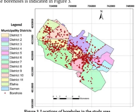
and geotechnical properties of soil was developed. The distribution of the boreholes is indicated in Figure 3.
Figure 3. Locations of boreholes in the study area.
The majority of the boreholes are located in the downtown, western and southern parts of the city while fewer investigations have been carried out in the northeastern part. The northeastern part of Mashhad includes very old buildings and there have not been many new constructions there. On the other hand, new high-rise buildings including residential complexes, hotels, shopping malls and governmental buildings have been centralized in western and northwestern parts of the city.
In this research, some geotechnical index properties including percentage of fine-grained material (grain size<0.075 mm based on ASTM D422), liquid limit (LL), and plasticity index (PI) of soil were employed. The values of these parameters have been specified through soil mechanical tests proposed by ASTM (American Society for Testing and Materials) standards. The percentage of fine-grained material is the fraction of soil passing sieve No.200. Based on Unified Soil Classification System (USCS), soil is called fine grained (silt and clay) when the fraction of soil passing No.200 sieve exceeds 50% and it is called coarse grained (gravel and sand) when this fraction is less than 50%. Liquid limit is defined as the minimum moisture content at which a soil will flow under its own weight. Plasticity index is the difference between liquid limit and plastic limit. It is a measure of the amount of water bounded within the sediment at specific stress or strength levels. Plastic limit (PL) is the percentage moisture content at which a soil can be rolled, without breaking, into a thread 3mm in diameter, any further rolling causing it to crumble. In other words, PL is defined as the moisture content at which soil begins to behave as a plastic material. LL and PI are representative of soil consistency and its plastic properties. These limits are influenced by the amount and character of the clay minerals content. Descriptive statistics of hard data related to each parameter is presented in Table 2.
Table 2. Descriptive statistical values of the parameters.
Parameter N Minimum Maximum Mean Std.
Deviation Variance
Fine-grained material 8330 0 100 35.67 31.586 997.663
PI 18070 0 33 3.79 4.915 24.160
LL 11333 0 69 23.28 9.709 94.274
4.
Geostatistical modeling
4.1.Spatial correlation analysis using variograms
The variogram, γ(h), measures the average dissimilarity between the values of a parameter (x) at location u and at a location u+h. Assuming stationarity, the variogram γ(z(u), z(u+h)) depends on a lag vector h: γ(h). The experimental variogram is calculated based on the following equation:
𝛾(ℎ) = 1
2𝑁∑ [𝑧(𝑢𝛼) − 𝑧(𝑢𝛼+ ℎ)] 2 𝑁
𝛼=1 (1)
Where z(u) is the value of the parameter at location u and N is the number of data pairs separated by vector h.
Analytical functions (called theoretical variograms) are used to model the experimental variograms to meet three main purposes: 1) they guarantee unique solutions, 2) they allow for the calculation of a variogram value, γ (h), for any given lag vector, h., and 3) they allow for filtering of the noise, which is usually a result of either imperfect measurements or lack of data. The most common theoretical variograms that can either be used by themselves or as nested structures in order to describe more complicated experimental variograms are as follows:
1. Spherical model with range a:
(ℎ) = { 3 2 ‖ℎ‖ 𝑎 − 1 2( ‖ℎ‖ 𝑎)
3 𝑖𝑓 ‖ℎ‖ ≤ 𝑎
1 𝑜𝑡ℎ𝑒𝑟𝑤𝑖𝑠𝑒 (2)
2. Exponential model with practical range a:
𝛾(ℎ) = 1 − exp (−3‖ℎ‖
𝑎 ) (3)
3. Gaussian model with practical range a:
𝛾(ℎ) = 1 − exp (−3‖ℎ‖2
𝑎2 ) (4)
The upper bound of a theoretical model is called the “sill.” The range is the lowest lag at which the variogram reaches the sill. The sill is reached asymptotically in the case of exponential and Gaussian models. The distance at which 95% of the sill is reached is called the “practical range.”
Since the geological data often display some degree of anisotropy, it is always beneficial to assess the possible effect of anisotropy on variograms in multiple directions. In this study, variogram modeling was performed on the normal score transformed data. Experimental variograms of normal scores were searched in various directions. Attention was given to find a model which would best fit each of the variograms. The number of lags, lag separation distances, and lag tolerance were different in each case, depending on the nature of data and the spatial correlations they demonstrate.
4.2.Variography Validation Using Cross-Validation
The cross-validation technique is applied to choose the best variogram model among different models and to select the search radius and lag distance that minimize the kriging variance. For cross-validation, interpolation is performed at all of the data points, ignoring in turn, each one of them one after the other. Then the estimated and true values are compared. Cross-validation checks how well the variogram model estimates the value of soil properties at an un-sampled location.
4.3.Sequential Gaussian Simulation (SGS)
Sequential simulation is a stochastic modeling algorithm that obtains multiple realizations based on the same input data [37-38]. These data could be either continuous or categorical. Considering the data type, one of the methods among sequential indicator simulation, Sequential Gaussian Simulation (SGS: [39-40]) or direct sequential simulation will be chosen. The most straightforward algorithm for generating realizations of a multivariate Gaussian field is presented by the sequential principle [31, 41-42]. In SGS method, data are transformed into Gaussian through a quantile transformation because it employs standard Gaussian data i.e. the ones with zero mean and unit variance [30]. Then, each variable is simulated sequentially based on its normal Complementary Cumulative Distribution Function (CCDF) using Simple Kriging (SK) estimation. The conditioning data consist of all original data and all previously-simulated values found within a neighborhood of the location being simulated [31, 41-42].
Sequential simulation formalism is used to simulate a Gaussian random function. Let Y(u) be a multivariate Gaussian random function with zero mean, unit variance, and a given variogram model γ(h). Realizations of Y(u) can be generated as follows [43]:
3- For each node u along the path:
Get the conditioning data consisting of original neighborhood hard data (n) and previously-simulated values.
Estimate the local conditional Cumulative Distribution Function (CDF) as a Gaussian distribution with mean given by kriging and variance by the kriging variance.
Draw a value from that Gaussian (CCDF) and add the simulated value to the data set.
4- Repeat the steps described in number 2 for another realization. When all the realizations are generated, the Gaussian simulated field is back-transformed into the data space (Y(u) → Z(u)) [32]. Regarding a transformation to Gaussian and then back-transform to an original unit, statistical fluctuations are inherent in simulation but the fluctuations should be reasonable and unbiased in the mean and variance [44]. The following checks should be performed after having all nodes simulated: reproduction of (1) the data values at data locations, (2) the original histogram, (3) the original summary statistics, and (4) the input covariance model [44].
5.
Results and discussion
5.1.Variability Analysis
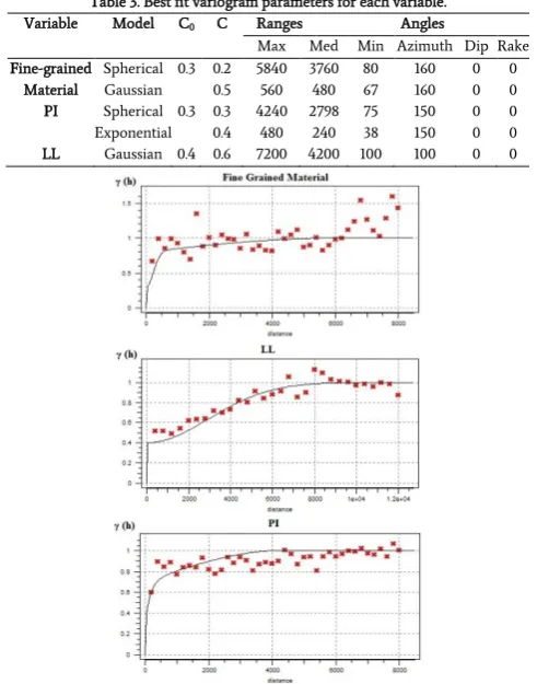
In order to identify variogram parameters and define a 3D search ellipsoid for each variable in this study, theoretical variogram functions were determined based on the experimental ones for each variable studied. Then, cross-validation was carried out to select the best fit variogram model. In this regard, the estimated values were drawn versus true ones. The best variograms of the parameters in their major axes of anisotropy are illustrated in Figure 4. Furthermore, the results of cross-validation for the best fit variogram model of each parameter are presented in Figure 5. The variogram model, nugget effect (C0), contribution (C), ranges, and angles were determined as variogram parameters resulting from theoretical variograms (Table 3).
Table 3. Best fit variogram parameters for each variable.
Variable Model C0 C Ranges Angles
Max Med Min Azimuth Dip Rake Fine-grained
Material
Spherical 0.3 0.2 5840 3760 80 160 0 0
Gaussian 0.5 560 480 67 160 0 0
PI Spherical 0.3 0.3 4240 2798 75 150 0 0
Exponential 0.4 480 240 38 150 0 0
LL Gaussian 0.4 0.6 7200 4200 100 100 0 0
Figure 4. Variograms of the parameters in their major axes.
Figure 5. Cross-validation results a: fine-grained material b: LL c: PI.. It is worth noting that initially a trend in the variogram related to the percentage of fine-grained material was recognized. Therefore, the data were first de-trended and then the final variogram for fine-grained material was calculated which is demonstrated in Figure 4. In order to de-trend these data, in the first step the percentage of fine-grained material versus the X direction was drawn and the relationship between these two was assessed and the equation was estimated. In the next step, the real values were subtracted from the model values which had been calculated based on the estimated equation.
5.2.Sequential Gaussian Simulation of the Parameters
In order to simulate the parameters under study, fifty realizations of each parameter were generated on 100×100×10 (m3) grids covering the study area. Simulation was performed using Simple Kriging estimator, and the variogram model for normal score transformed data. In addition, uncertainty assessment was done by determination of Coefficient of Variation (CV) related to the simulation results. CV is calculated based on the following equation:
𝐶𝑉 =𝜎
𝜇 (5)
of all realizations.
Moreover, E-type maps which are in fact smoother versions of realizations and are drawn by averaging all realizations, were prepared.
5.2.1.Fine-grained Material
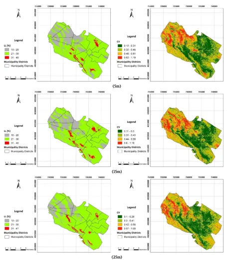
The amount of fine-grained material (silt and clay) plays a significant role in geotechnical properties of soil and recognition of different sedimentary environments. So, the 3D model of fine-grained material was developed for Mashhad soil based on SGS approach in order to be employed as a base model in geological and geotechnical interpretations (Figure 6). According to Figure 6, an obvious increasing trend toward east and northeast can be recognized in the percentage of fine-grained material. Generally speaking, in the eastern part of the city, subsurface soil is categorized in C and M groups based on Unified Soil Classification System while in the western part, it falls in G and S groups. Moreover, the particle size of soil expands with the increase in depth. Maps of E-type along with CV are depicted in Figure 7 for the soil depths of 5 m, 15 m, and 25 m of the studied area. The same trend is clearly visible in E-type map presented in Figure 7. An increase in CV value can be a result of inadequate conditional data and/or high degree of
heterogeneity. Since the opposite trend is recognizable in the CV map shown in Figure 7, it can be concluded that homogeneity in soil texture increases toward northeast of the study area because of the shortage of data and it may not typically follow such pattern. The presence of recent alluviums in western areas might be the main reason of higher heterogeneity there; while moving through the flat plain which is representative of a flood plain environment, brings about a more homogeneous condition and consequently the CV values decrease.
Figure 6. 3D model of fine-grained material (average values) in Mashhad soil in oblique view with vertical exaggeration coefficient equals 10.
(5m)
(25m)
Figure 7. E-type map (left) and CV map (right) of fine-grained material.
Considering the geological viewpoint and based on Figure 2, the source of alluvial sediments in Mashhad basin is commonly from the western and southern alluvial fans especially Chel Baze fan. The observed trend in the percentage of fine-grained material confirms this hypothesis.
5.2.2.Plasticity Limits
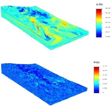
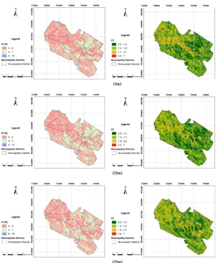
Plasticity limits are in close relationship with the amount of fine-grained material as well as type of clay mineral. 3D models for plasticity limits (PI) and liquid limits (LL) of Mashhad soil are demonstrated in Figure 8. Moreover, E-type and CV maps related to PI and LL are presented in Figures 9 and 10, respectively.
According to the high percentage (>50%) of fine-grained material in eastern and northeastern parts of Mashhad, it might be expected that values of PI as well as LL would be high in those areas. But as it is clear in figures number 8, 9, and 10, the values are not that high in those areas. Two reasons may be put forward for this phenomenon: high amount of clay-size soil (rock powder) and/or low activity clay soil. Presence of clay-size soil reflects a long transportation distance which in the case of present study area, it is not in harmony with the evidence. Transportation distance between western and southern sources of Mashhad sediments and the eastern deposition areas is not long enough to produce high amounts of clay-size particles. So it can imply that subsurface soil in eastern and northeastern parts of the city commonly consists of low plastic clay minerals such as Kaolinite and Illite. This result attests the previous findings on the types of clay minerals in Mashhad area [45].
Although PI values do not demonstrate intense variations, the values are generally lower in the western areas while higher in the eastern parts. Moreover, the approximately non-plastic long area in the middle of the PI model follows the path of recent alluvium originating from the western fans. Similar path can be distinguished in LL model. Recent alluvium consists of coarse-grained material. Regarding the CV map, more variations are observed compared with the CV map of fine-grained material.
As it can be inferred from Figure 10, variations of LL values in western parts of the city follow general form of Chel Baze alluvial fan (See Figure 2). The observed periodicity of LL values in those areas is a result of discharge changes in the main river of the fan due to changing climate conditions. Additionally, a long narrow area with higher values of LL is clearly recognizable along the southern margin of Mashhad. The dominant rock types in the west and southwest of Mashhad are slate and phyllite whereas ultrabasic rocks are widespread in the southern parts. Since weathering of ultrabasic rocks rather than metamorphic ones produce more active clay minerals, this narrow area may be a result of southern ultrabasic rocks weathering most probably.
Figure 8. 3D models of Mashhad soil plastic properties (average values) in oblique view with vertical exaggeration coefficient of 10.
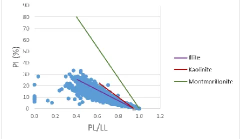
In addition, in Figure 11 the PI values were drawn versus the ration of PL to LL. This graph is representative of different sources of sediments in a region and different sedimentary environments. When different main sources are involved, various trends are observed in PI-PL/LL graph [46].
According to Figure 11, the data are accumulated along a single line; so it can be implied that Mashhad soil sediments have been originated from one main type of source which is believed to be western and southern alluvial fans. The source of these fans is ultrabasic and metamorphic rocks of Mount Binalud. The observed trend in the model of fine-grained material in the city seems to corroborate this hypothesis. Moreover, it can be seen that the soil in the study area consists of low-plasticity clay minerals e.g. illite and kaolinite.
5.2.3.Data Analysis on the Simulation Results
conclusion that the distribution of the original data is so similar to the one from simulated results.
(5m)
(15m)
(25m)
(5m)
(15m)
(25m)
Figure 10. E-type map (left) and CV map (right) of liquid limit.
Table 4. Descriptive statistics of the simulated parameters.
Parameter N Minimum Maximum Mean Std. Deviation Variance
E-type (Fine-grained material) 590202 1.9 95.4 35.63 23.192 537.872
Real 0 (Fine-grained material) 590202 0 100 35.63 31.585 997.583
E-type (PI) 590202 0 17.8 3.78 0.793 0.629
Real 30 (PI) 590202 0 33 3.78 4.904 24.052
E-type (LL) 590202 9.7 40.6 23.25 2.708 7.332
Real 15 (LL) 590202 0 69 23.25 9.707 94.223
In addition to comparisons of basic statistical parameters outlined above, Q–Q plots which are used to compare probability distributions, were prepared for each simulated parameter for their hard data versus a random realization. A straight line is an indication of equality between
figure displays that comparisons of simulated data offer nearly linear relationships with the hard data from which they are generated, and thus the probability distributions of all data are almost identical.
Figure 11. Investigation of sediments source in Mashhad municipal area.
Figure 12. Q-Q plots of the hard data against a random realization.
6.
Conclusions
This study which is regarded as the first comprehensive research on geotechnical index parameters of Mashhad soil sediments, will be hopefully useful for future research as well as ongoing civil engineering projects. Moreover, it can suggest the appropriate and efficient location of future investigation boreholes. For the sake of brevity, the main results of this study can be summarized as follows:
1- Variability analyses were conducted on three index properties of soil in Mashhad municipal area, i.e., the percentage of fine-grained material, liquid limit, and plasticity index.
2- Mashhad sedimentary deposits consist of a wide and varied range of fine- to coarse-grained soil. In Mashhad, the amount of fine-grained material increases toward eastern and northeastern parts while it generally decreases in deeper layers. Since some eastern parts of the city are being renovated and old buildings are to be replaced with high-rise and modern ones, necessary and appropriate precautions related to fine-grained soil should be taken into consideration from an engineering point of view. 3- The presence of recent alluviums in western areas has led to
higher heterogeneity there while a more homogeneous condition is dominant in central and eastern parts of the city. 4- It seems that the sources of alluvial sediments in Mashhad basin
are commonly from the western and southern alluvial fans especially Chel Baze fan. The observed trend in the percentage of fine-grained material coupled with the PI versus PL/LL graph is in agreement with this hypothesis.
5- Subsurface soil in the city commonly consists of low-plasticity clay minerals. PI values are generally lower in the western areas while higher in eastern parts.
6- The approximately non-plastic long areas in the middle of the PI and LL model follow the path of recent alluvium originated from the western fans.
7- Variations of LL values in western parts of the city derive from Chel Baze Alluvial Fan. In addition, the long narrow area with higher values of LL along the southern margin of Mashhad is probably a result of the weathering of southern ultrabasic rocks. 8- According to the comparison made between the descriptive
statistics of simulated data and original data coupled with the Q-Q plots, the probability distributions of all data including simulated and original ones are so similar. Thus, it can be inferred that the results of simulations are reasonably reliable.
Acknowledgement
The authors would like to gratefully thank the Iranian Organization for Engineering Order of Building (Khorasan Razavi province) for supplying us with borehole data. Furthermore, the authors hereby acknowledge that parts of the computations were performed on the high-speed systems at the High-Performance Computing (HPC) Center, Ferdowsi University of Mashhad.
REFERENCES
[1] Shepherd, R. G. (1989). Correlations of permeability and grain size. Ground Water, 27, 633-638.
[2] Arya, L. M., Leij, F. J., Shouse, P. J., & Van Genuchten, M. Th. (1999). Relationship between the hydraulic conductivity function and the particle-size distribution. Soil Sci. Soc. Am. J., 63, 1063-1070.
[3] Price, D. G. (2009). Engineering geology, principles and practice. Springer-Verlag Berlin/Heidelberg, 450 p.
direct shear tests for clay-sand mixtures. Adv. Mater. Sci. Eng. http://dx.doi.org/10.1155/2013/562726.
[5] Bell, F. G. (2007). Engineering Geology. 2nd edition, Elsevier, 581 p.
[6] De Rienzo, F., Oreste, P., & Pelizza, S. (2008). Subsurface geological-geotechnical modeling to sustain underground civil planning. Eng. Geol., 96, 187-204.
[7] Royse, K. R., Rutter, H., & Entwisle, D. (2009). Property attribution of 3d geological models in the Thames gateway, London: New ways of visualizing geoscientific information. B. Eng. Geol. Environ., 68, 1–16.
[8] Tonini, A., Guastaldi, E., Massa, G., & Conti, P. (2008). 3D geo-mapping based on surface data for preliminary study of underground works: a case study in Val Topina (Central Italy). Eng. Geol., 99, 61-69.
[9] De Beer, J., Price, S. J., & Ford, J. R. (2012). 3D modeling of geological and anthropogenic deposits at the World Heritage Site of Bryggen in Bergen, Norway. Quatern. Int., 251, 107-116. [10] Tame, C., Cundy, A. B., Royse, K. R., Smith, M., & Moles, N. R.
(2013). Three-dimensional geological modeling of anthropogenic deposits at small urban sites: A case study from Sheepcote Valley, Brighton, UK. J. Environ. Manage., 129, 628-634.
[11] Mathers, S. J., Burke, H. F., Terrington, R. L., Thorpe, S., Dearden, R. A., Williamson, J. P., & Ford, J. R. (2014). A geological model of London and the Thames Valley, southeast England. Proceedings of the Geologists’ Association, 125, 373-382. [12] Touch, S., Likitlersuang, S., & Pipatpongsa, T. (2014). 3D
geological modeling and geotechnical characteristics of Phnom Penh subsoils in Cambodia. Eng. Geol., 178, 58-69.
[13] Kim, Y. Y., & Lee, K. K. (2002). Construction and interpretation of a hydrogeological data base for the Seoul groundwater system. Geosci. J., 6, 319-330.
[14] Kessler, H., Mathers, S., & Sobisch, H. G. (2009). The capture and dissemination of integrated 3D geospatial knowledge at the British Geological Survey using GSI3DTM software and methodology. Comput. Geosci., 35, 1311-1321.
[15] Royse, K. R., Reeves, H., & Gibson, A. (2008). The modeling and visualization of digital geoscientific data as an aid to land-use planning in the urban environment, an example from the Thames Gateway. In: Liverman D, Pereira C, Marker B (Eds.), Communicating Environmental Geoscience. Special Publication 305, Geological Society of London, 89-106.
[16] Royse, K. R. (2010). Combining numerical and cognitive 3D modeling approaches in order to determine the structure of the Chalk in the London Basin. Comput. Geosci. 36, 500-511. [17] Stafleu, J., Maljers, D., Gunnink, J. L., Menkovic, A., & Busschers,
F. S. (2011). 3D modeling of the shallow subsurface of Zeeland, the Netherlands. Neth. J. Geosci., 90, 293-310.
[18] De Beer, J., Matthiesen, H., & Christensson, A. (2012). Quantification and visualization of in situ degradation at the World Heritage Site of Bryggen in Bergen, Norway. Cons. Manage. Archael. Sites, 14, 215-227.
[19] Marinoni, O. (2003). Improving geological models using a combined ordinary-indicator kriging approach. Eng. Geol., 69, 37-45.
[20] Marache, A., Breysse, D., Piette, C., & Thierry, P. (2009). Geotechnical modeling at the city scale using statistical and geostatistical tools: The Pessac Case (France). Eng. Geol., 107, 67-76.
[21] Lee, W., Kim, D., Chae, Y., & Ryu, D. (2011). Probabilistic evaluation of spatial distribution of secondary compression by using kriging estimates of geo-layers. Eng. Geol., 122, 239-248.
[22] Parvin, M., Tadakuma, N., Asaue, H., & Koike, K. (2011). Characterizing the regional pattern and temporal change of groundwater levels by analyses of a well log data set. Front. Earth Sci., 5, 294-304.
[23] De Carvalho, L.A., Meurer, E., Da Silva Junior, C.A., Santos, C. F. B., & Libardi, P. L. (2014). Spatial variability of soil potassium in sugarcane areas subjected to the application of vinasse. An. Acad. Bras. Ciênc., 86, 1999-2012.
[24] Ozturk, C.A., & Simdi, E. (2014). Geostatistical investigation of geotechnical and constructional properties in Kadikoy-Kartal subway, Turkey. Tunn. Undergr. Sp. Tech., 41, 35-45.
[25] Tripathi, R., Nayak, A. K., Shahid, M., Raja, R., Panda, B. B., Mohanty, S., Kumar, A., Lal, B., Gautam, P., & Sahoo, R. N. (2015). Characterizing spatial variability of soil properties in salt affected coastal India using geostatistics and kriging. Arab. J. Geosci., 8, 10693-10703.
[26] Negreiros, J., Painho, M., & Aguilar, F. (2008). Principles of deterministic spatial interpolators. Polytechnical Studies Review, 6, 1–11.
[27] Bourgine, B., Dominique, S., Marache, A., & Thierry, P. (2006). Tools and methods for constructing 3d geological models in the urban environment: The case of bordeaux. In IAEG.
[28] Krige, D. (1951). A statistical approach to some basic mine valuation problems on the witwatersrand. Journal of the Chemical, Metallurgical and Mining Society of South Africa, 52, 119–139.
[29] Matheron, G. (1963). Principles of geostatistics. Economic Geology, 58, 1246–1266.
[30] Chilès, J. P. & Delfiner, P. (2012). Geostatistics: Modeling Spatial Uncertainty. 2nd edition, Wiley, 734 p.
[31] Leuangthong, O., McLennan, J. A., & Deutsch, C. V. (2004). Minimum acceptance criteria for geostatistical realizations. Nat. Resour. Res., 13, 131–141.
[32] Deutsch, C., & Journel, A. G. (1998). GSLIB: Geostatistical Software Library and User's Guide. 2nd Edition, Oxford University Press, New York, 369 p.
[33] Goovaerts, P. (1997). Geostatistics for Natural Resources Evaluation. Oxford University Press, New York, 483 p. [34] Delbari, M., Afrasiab, P., & Loiskandl, W. (2009). Using
Sequential Gaussian Simulation to assess the field-scale spatial uncertainty of soil water content. Catena, 79, 163–169.
[35] Nikpeyman, V. (2014). Simulating the Effect of Water Supplying from Doosti Dam on the Part of the Mashhad’s Aquifer Located in City Limit Using MODFLOW. M.Sc. Thesis, Ferdowsi University of Mashhad, Mashhad, Iran, 136 p. (in Persian with English abstract)
[36] Ghazi, A., Hafezi Moghadas, N., Sadeghi, H., Ghafoori, M., & Lashkaripour, G. (2015). The effect of geomorphology on engineering geology properties of alluvial deposits in Mashhad City. Scientific Quarterly J., Geosciences, 24, 17-28. (in Persian with English abstract)
[37] Geboy, N. J., Olea, R. A., Engle, M. A., & Martín-Fernández, J. A. (2013). Using simulated maps to interpret the geochemistry, formation and quality of the Blue Gem coal bed, Kentucky, USA. Int. J. Coal. Geol., 112, 26–35.
[38] Journel, A. G. (1993). Modeling Uncertainty: Some Conceptual Thoughts, Geostatistics for the Next Century. Kluwer Academic Publications, 30-43.
[41] Manchuk, J. G., & Deutsch, C. V. (2012). Implementation aspects of Sequential Gaussian Simulation on irregular points. Comput. Geosci., 16, 625–637.
[42] Manchuk, J. G., & Deutsch, C. V. (2012). A flexible Sequential Gaussian Simulation program: USGSIM. Comput. Geosci., 41, 208–216.
[43] Remy, N., Boucher, A., & Wu, J. (2009). Applied Geostatistics with SGeMS. Cambridge University Press, 264 p.
[44] Zanon, S., & Leuangthong, O. (2004). Implementation aspects of sequential simulation. In: Leuangthong O, Deutsch C (Eds.), Geostatistics Banff, vol. 1. Springer Science + Business Media 543–550.
[45] Yousefi, E., Lashkaripour, G., Ghafoori, M., & Talebian, L. (2008).
Investigation of clay minerals in Mashhad City based on their Atterberg Limits. Proceeding of the 5th Iranian Conference of Engineering Geology and Environment, 914-920. (in Persian with English abstract)
[46] Moradi Harsini, K. (2008). Relationship between Geological Engineering Properties of Recent Sedimentary Deposits and Sedimentary Environment in Khouzestan Plain Using Satellite Images. Ph.D. Dissertation, Tarbiat Modarres University, Tehran, Iran, 387 p. (in Persian with English abstract) [47] Krishnamoorthy, K. (2006). Handbook of statistical distributions