__________
* Corresponding author
E-mail addresses:[email protected](P. Jamshidi);[email protected](H. Rastiveis)
website: https://eoge.ut.ac.ir
Extraction of ground points from LiDAR data based on slope and
progressive window thresholding (SPWT)
Pejman Rashidi, Heidar Rastiveis*
School of Surveying and Geospatial Engineering, College of Engineering, University of Tehran, Tehran, Iran
Article history:
Received: 22 August 2017, Received in revised form: 10 March 2018, Accepted: 1 April 2018 ABSTRACT
Filtering of airborne LiDAR point clouds has broad applications, such as Digital Terrain Model (DTM) generation and three-dimensional urban modeling. Although several methods have been developed to separate the point clouds into ground and non-ground points, there are some challenges to identify the complex objects such as bridge and eccentric roofs. In this study, a new algorithm based on the Slope and Progressive Window Thresholding (SPWT) is proposed for ground filtering of LiDAR data. This algorithm is based on both multi-scale and slope methods that have strong effects on filtering the LiDAR data. The proposed algorithm utilizes the slope between adjacent points and the elevation information of points in a local window to detect non-ground objects. Therefore, not only it benefits from vertical information in each local window to detect the non-ground points, but it also uses the neighbor information in directional scanning, and it prevents the errors introduced by the sensitivity to direction. According to the physical characteristics of the ground surface and the size of objects, the best threshold values are considered. In order to evaluate the performance of the SPWT method, both low and high resolution datasets were applied that their average overall accuracy were reported to be 94.21% and 93.08%, respectively. These results proved that, irrespective of data resolution, the SPWT method could effectively remove the non-ground points from airborne LiDAR data.
S
KEYWORDS
Ground Filtering LiDAR Point clouds DTM Generation
1. Introduction
Airborne light detection and ranging (LiDAR) is one of the most popular technologies to rapidly gather the three-dimensional coordinates of ground and non-ground objects, such as buildings, trees, vehicles, and so on. LiDAR has several advantages over the traditional field surveying and photogrammetric mapping, e.g., cost-effective coverage of a large area for acquisition of vertical information, higher accuracy, gathering information in all types of weather, season and it does not depend on time in data collection (Meng et al., 2009; Shan & Aparajithan, 2005; Li et al., 2014; Zhang & Whitman, 2005).
Digital Terrain Model (DTM) generation is one of the most popular applications of the LiDAR data (Bretar & Chehata 2010; Zhang & Lin, 2013; White & Wang, 2003), which is a three-dimensional model indicating the spatial
distribution of the earth’s surface (Quan et al., 2016). In DTM generation from the LiDAR data, the first step is separating the ground and non-ground points, a process referred to as filtering (Li, 2013; Li et al., 2013), and the non-ground points should be removed from LiDAR’s measurements (Vosselman, 2000).
73 In order to identify the ground points, some approaches
work on the raw LiDAR point clouds. Although these methods have certain advantages, e.g., they require less preprocessing, finding the neighboring points in an irregularly distributed space can be a time-consuming process, especially for large areas. Therefore, in many filtering methods, the point clouds are resampled into a gridded elevation model to resolve this problem, however interpolation may introduce some errors (Sithole & Vosselman, 2004; Meng et al., 2009). For resampling the point clouds into a regular grid data, multiple interpolation techniques have been introduced, which can be divided into three categories: fitting a 1.morphology function (Chen et al., 2007) 2.linear function (Andersonet al., 2005) 3.surface function (Okagawa, 2001).
There are different types of methods for filtering the LiDAR data that the most important of which are based on a. Triangulated Irregular Network (TIN) b. Slope c. Morphological approaches d. Multi-scale comparison.
Some algorithms are based on triangulated irregular network, and search for neighboring points by creating a TIN with certain constraints of angle and distance (Axelsson, 2000; Uysal & Polat, 2014). (Quan et al., 2016) utilized the adjacent triangle of a triangulated irregular network to detect the building edge points, and get the building points by the region growth. Afterward, the isolated points were detected through the morphological filtering algorithm. This algorithm was tested only on urban areas and no results have been reported for rural areas.
Most of ground filters are based on the slope between the neighboring points. In these approaches, the points are labeled as ground and non-ground based on a pre-defined threshold value (Sithole, 2001; Wang & Tseng 2010). Usually, selecting the best threshold value is a significant and challenging parameter. (Susaki, 2012) used the slope threshold that was dynamically tuned according to the terrain. In this method, the ground points could be extracted with a good accuracy in urban areas, but the computation time is long.
The morphological algorithms have been applied for filtering the LiDAR data by many researchers. They have simple concepts and are able to eliminate the non-ground objects (Arefi & Hahn, 2005; Kobler et al., 2007). (Zhang et al., 2003) compared the height differences of original and morphologically opened surfaces with an appropriate threshold, and determined the non-ground objects progressively with increasing the window size. (Li et al., 2014) improved the top-hat morphological filter with a sloped brim. The intensity of change elevation of transitions between the obtained top-hats and outer brims were assessed to suppress the omission error caused by protruding terrain features, and finally, the non-ground objects were identified by the brim filter, that was extended outward.
Several algorithms are based on multi-scale comparison. These methods produce some preliminary trend surfaces and each point is examined at different scales by comparing the elevation difference between the point and different trend surfaces (Chen et al., 2017; Zhang & Whitman, 2005). These methods provide practical and reliable solutions for integrating merits of DTM generated using different methods (Chen et al., 2017). (Chen et al., 2012) proposed an upward-fusion DTM generation method. In their technique, some preliminary DTMs of different grid sizes are produced using the local minimum method. Then, an upward fusion is conducted between these DTMs. This algorithm begins with a DTM of the largest grid size and a finer scale DTM is compared with that.
From the aforementioned studies, it can be concluded that although several methods have been proposed for filtering the LiDAR point clouds, a powerful method has not yet been developed to be able to eliminate all objects from the LiDAR data. Therefore, filtering the LiDAR point clouds can be known as an open problem in photogrammetry and remote sensing. In this study, we have proposed a novel method based on the slope and progressive window thresholding for filtering the LiDAR point clouds. Progressive windows include two windows, the first one removes the small non-ground objects such as shrubs, and the second window eliminates the large objects such as buildings. In addition, the slope between two neighbor pixels can remove high outliers and the edge of the buildings. According to the physical characteristics of the ground surface and the size of objects, the best threshold value is considered. In the following, the paper explains the basic procedure of this algorithm and presents results and analyses obtained from its implementation.
2. Proposed Method
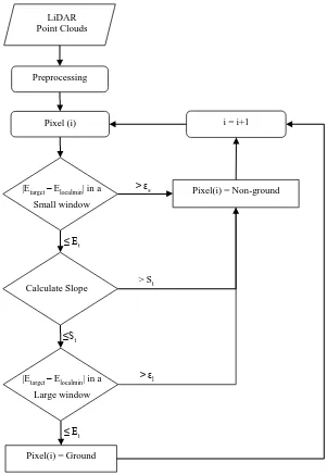
In this paper, a new method for filtering the LiDAR data is proposed based on the slope and progressive window thresholding (SPWT). The flowchart of the SPWT method is shown in Figure 1. As shown, the non-ground points are eliminated through four main steps: preprocessing, small window thresholding, slope thresholding, and large window thresholding.
73 and its neighbor pixels, the non-ground pixels are detected,
which have not been previously recognized. The last step is the same as the aforementioned step, but it is in a larger window size. Actually, the elevation difference between the candidate pixel and the minimum elevation of the local window is calculated. If the difference value exceeds from a predefined threshold, the candidate pixel is labeled as non-ground point.
The window sizes are specified from the smallest to the largest objects in the area. In addition, according to the physical characteristics of the ground surface and the size of objects, the best height threshold is selected manually. Furthermore, the slope threshold should be assigned based on the topographical condition of the area.
The SPWT method selects the pixels in order from the first to the last scan line, and after finding the ground seed, the algorithm iterates repeatedly through the following steps to the label points as ground or non-ground. The main steps
of the proposed method are described in more details in the following sections.
2.1 Preprocessing
In this study, two preprocessing steps are necessary before applying the SPWT algorithm: resampling the LiDAR point clouds and outlier removal. The aim of resampling is to convert the irregular point clouds into a regular distributed grid through an interpolation technique. Here, the nearest neighbor technique that considers the elevation of the nearest point in a specified distance to the output pixel is performed. If no points were observed in the specified distance, the pixel would be labeled as no data. Therefore, to avoid too many or no points in each grid cell, the size should be determined by the average point spacing of the point clouds (Li et al. 2014). After resampling the points into a regular distributed grid, the outliers should be removed from the data. In the LiDAR data, the outliers are points with abnormal elevation values, Preprocessing
Pixel(i) = Ground Pixel (i)
Pixel(i) = Non-ground i = i+1 LiDAR
Point Clouds
|Etarget – Elocalmin| in a
Small window
Calculate Slope
|Etarget – Elocalmin| in a
Large window
> εs
> St
> εl ≤ Et
≤St
≤ Et
73 either higher or lower than the surrounded points. The
outliers with high elevation values, which usually include random errors and result from birds or airplanes, are usually eliminated during the filtering process, because they can be assumed as non-ground objects. While, low outliers are below the surface and may be resulted from several times reflecting of laser returns. These outliers may seriously affect the filtering results. Therefore, they should be removed from the data in the preprocessing step (Li et al., 2013). In this study, we used a rank value to remove the low outliers (Eckstein & Muenkelt, 1995),which can be alternative low outliers with a median of gray value in a local window. We consider 𝐺𝑝 be the gray values of a local neighborhood of pixel p, and n=|Gp | be the number of pixels in the local window. The gray values Gip∈Gp .i∈1…n are sorted by a function s in Eq. (1).
Gs(1)p ≤… ≤ Gs(n)p (1)
After sorting the gray values, the points at the end of gray values with abnormal lower gray values could potentially be outliers and are replaced by the median of the sorted gray values.
2.2 Small Window Thresholding
After the preprocessing step, the small non-ground objects, such as shrubs, vehicles and small trees that have a further height compared with their neighbors range are removed in the small window thresholding step. To identify these types of non-ground pixels, the elevation difference between these pixels and the minimum elevation in a local window is calculated. Meanwhile, depending on the size and the height of the objects in the area, height difference threshold should be assigned. Also, the window size in this step is based on the smallest object in the area.
This approach may not work on some pixels, and if the elevation difference is less than or equal to the height difference threshold, the pixel should be checked in the next steps. Therefore, more investigations are required to detect the non-ground pixels.
2.3 Slope Thresholding
In this step, the slope between each pixel and the previous pixel is calculated, and the candidate pixel would be labeled as a non-ground point if the slope were larger than a predefined threshold value. As well, it proceeds to the next step if the slope is less than or equal to the threshold value. The slope angle 𝜃 can be calculated according to the Eq. (2).
θ= tan-1 ( |z
2- z1| /√(x2- x1)2+ (y2- y1)2 ) (2) where x1, y1, z1and x2, y2, z2 are the coordinates for arbitrary points. In this case, the points that have vivid height differences in comparison with the previous point could be
identified as non-grounds such as noises and the edge of the buildings. The slope threshold should be assigned based on the topographical condition of the area. Although, this step and the previous one are highly capable to eliminate the small objects, they will not be able to remove larger objects such as buildings and bridges. In these cases, the height and slope of the central points are not locally changed. Therefore, considering a larger window search is necessary to remove the central points.
2.4 Large Window Thresholding
In the last step, a large window is considered to remove the central points of the large non-ground objects such as buildings or bridges. The processes in this step are mostly similar to the small window thresholding step, but there are two main differences:
1. The window size. The small window thresholding step
cannot identify large objects, since the size of window is not large enough to cover them completely, and there is no ground seed for calculating the height difference between the ground and the object. Therefore, a larger window is needed to detect the large objects.
2. The height difference threshold. In the small window,
small objects with low height value can be removed, but it is not appropriate for objects with high elevation values such as buildings. Therefore, to remove these objects, the height difference threshold should be adjusted.
Therefore, the window size and the height difference threshold should be adjusted in this step. Meanwhile, the window size is defined based on the largest object, so it may differ in each dataset. In addition, the height difference threshold value would be defined based on the height of large objects.
3. Data
In this study, in order to evaluate the performance of the SPWT algorithm, two datasets with different spatial resolution were tested. The details of these datasets are described in the following sections.
3.1 Low Resolution Datasets
The first dataset is the benchmark dataset provided by the International Society for Photogrammetry and Remote
Sensing (ISPRS) Commission III/WG3
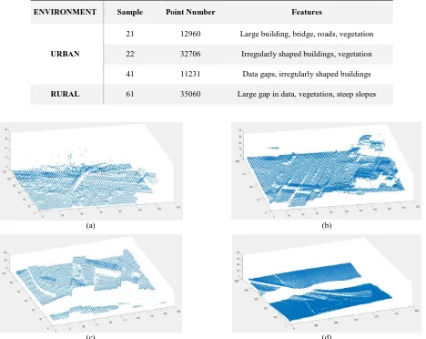
(http://www.itc.nl/isprswgIII-3/filtertest/). This paper chose the sample datasets included the typical urban and rural areas with different complex features, which are sample_21, sample_22, sample_41 and sample_61. The characteristics of these samples are shown in Table 1. In addition, the reference datasets were provided by the ISPRS using semi-automatic and manually filtering with recognition landscape and the aerial images (Chen et al., 2013). The LiDAR point clouds of these samples are depicted in Figure 2.
04
ENVIRONMENT Sample Point Number Features
URBAN
21 12960 Large building, bridge, roads, vegetation
22 32706 Irregularly shaped buildings, vegetation
41 11231 Data gaps, irregularly shaped buildings
RURAL 61 35060 Large gap in data, vegetation, steep slopes
(a) (b)
(c) (d)
Figure2. LiDAR point clouds. (a) Sample 21, (b) Sample 22, (C) Sample 41, and (d) Sample 61
Figure 3.LiDAR points cloud from IEEE with high resolution
3.2 High Resolution Dataset
Today, due to the development of the LiDAR technology, the density of collected point clouds is arising (Zhang et al., 2016). Thus, in this research, a high-resolution dataset was tested to have a better evaluation of the SPWT algorithm. This dataset was provided by (IEEE, 2015), and was cropped as part of the urban area in Zeebruges, Belgium with an average point density of 65 points/m2, which is related to a point spacing of approximately 10 cm. The LiDAR point
clouds of this sample is shown in Figure 3. As shown, this dataset covers various terrain types including irregularly shaped buildings with eccentric roofs, roads, vehicles and vegetation. In addition, an expert manually generated the ground truth for this sample.
4. Experiment and results
In this study, the SPWT algorithm was implemented using MATLAB R2015b. In the following, the results are discussed and evaluated.
4.1 Filtering validation
04 Table 2.Parameter values in the SPWT algorithm for filtering the low resolution LiDAR dataset
Datasets Size of small
window
Height difference
threshold in small
window
The slope
threshold
Size of large
window
Height difference
threshold in large
window
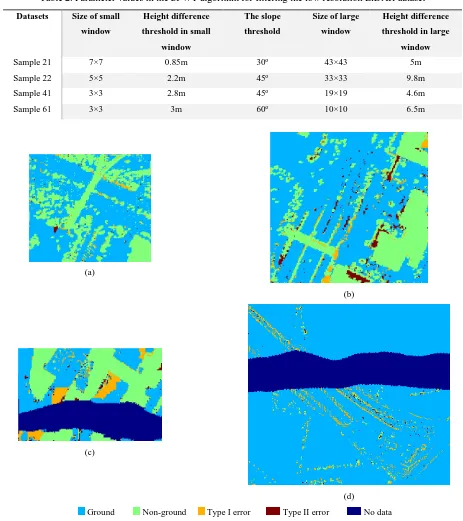
Sample 21 7×7 0.85m 30o 43×43 5m
Sample 22 5×5 2.2m 45o 33×33 9.8m
Sample 41 3×3 2.8m 45o 19×19 4.6m
Sample 61 3×3 3m 60o 10×10 6.5m
(a)
(b)
(c)
(d)
Ground Non-ground Type I error Type II error No data
Figure 4. Error distribution in filtering of the low resolution LiDAR datasets. (a) Sample 21, (b) Sample 22, (C) Sample 41 and (d) Sample 61
In the next step, five parameters were used for testing the algorithm, including the window size and the height difference threshold values for both small and large windows, and a threshold value in the slope thresholding step. Table 2 summarizes the applied parameters in testing the algorithm using the ISPRS benchmark dataset.
To evaluate the efficiency of the SPWT method, in this research, three indexes of error type I, error type II and total errors were used. If (a) is the total number of ground points,
04
al., 2009), the SPWT method showed a high performance in bridge identification. In sample 22, Figure 4(b), the irregularly shaped buildings and vegetation are well filtered, but many errors of type II are distributed around the buildings, which it means some of the pixels were incorrectly labeled as ground pixels. The reason may be abrupt changes in the height of the building roof. As it is clear in Figure 4(c), the proposed algorithm shows a decent effect on the irregularly shaped buildings with eccentric roofs in sample 41. However, a number of type I error points are observed in this sample. In sample 61, as it can be seen from Figure 4(d), there are a lot of type II errors distribute along steep slopes, because there are more dramatic ground surface changes in this area. Table 3 shows the calculated type I, type II, and the total errors for the test samples. As shown in this table, the minimum total error was observed in sample 21. Although this sample includes different objects, the SPWT algorithm successfully filtered these objects with low-level resulted type I, type II and total error rates. On the other hand, filtering sample 41 had the most significant total error, because this sample had many complex objects in comparison with other samples. Experimental results showed that the SPWT method can filter special features such as bridge, irregularly shaped buildings with eccentric roofs and low height vegetation, but it may have some errors in steep slopes. 4.2. Comparison and Discussion
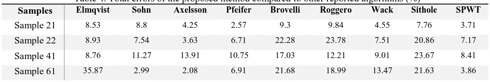
A large number of researchers have used the ISPRS dataset to evaluate their filtering algorithms. In this study, to quantitatively analyze the accuracy of the SPWT algorithm, the resulted of the total error from the proposed method was compared to eight other methods that were tested by the ISPRS (Sithole & Vosselman, 2003) dataset. The total errors of these samples are summarized in Table 4.
As Table 4 provides, the accuracy of the SPWT method is close to the other top filtering algorithms, except sample 22. Type II error for sample 22 distributed the surrounding of the buildings and is relatively high.
Moreover, the overall accuracy, which indicates the percentage of the properly classified points in all points (Hui et al., 2016), was calculated for the sample datasets. Figure 5 shows the average overall accuracy of filtering the test samples through the SPWT algorithm and the other previous
method shows the highest overall accuracy for these samples. In addition, there is a slight difference between the proposed method and the Axelsson algorithm, and a big difference in comparison with the Sithole algorithm.
Some other novel methods have proposed their new filtering algorithms in recent years, which use the samples provided by the ISPRS to evaluate their performance. The average total errors for four samples of these algorithms are shown in Table 5. As it is clear in this table, the SPWT method shows a decent performance in the LiDAR point clouds filtering. The average total error of the proposed method was only 0.65% higher than the lowest one.
Table3. Accuracy indexes for ISPRS dataset in the SPWT algorithm
Sample Dataset
TYPE I ERROR(%)
TYPE II ERROR(%)
TOTAL ERROR(%)
Sample 21 3.49 5.12 3.71
Sample 22 4.43 18.03 7.17
Sample 41 12.78 3.38 8.41
Sample 61 3.57 20.22 3.86
Figure 5. Average overall accuracy of the SPWT algorithm and the previous technique
Table 4. Total errors of the proposed method compared to other reported algorithms (%)
Samples Elmqvist Sohn Axelsson Pfeifer Brovelli Roggero Wack Sithole SPWT
Sample 21 8.53 8.8 4.25 2.57 9.3 9.84 4.55 7.76 3.71
Sample 22 8.93 7.54 3.63 6.71 22.28 23.78 7.51 20.86 7.17
Sample 41 8.76 11.27 13.91 10.75 17.03 12.21 9.01 23.67 8.41
Sample 61 35.87 2.99 2.08 6.91 21.68 18.99 13.47 21.63 3.86
0% 10% 20% 30% 40% 50% 60% 70% 80% 90% 100%
84.43%92.35% 94.03%
93.27%
82.43%83.8% 91.37%
07 4.2 Testing the high resolution LiDAR data
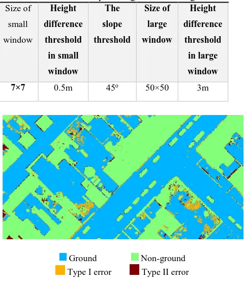
The SPWT method was also tested by a high-resolution dataset. Table 6 summarizes the applied parameters in testing the algorithm using the IEEE dataset. In resampling of this dataset, the pixel size was considered 0.2 meter. Moreover, this dataset contains types of objects in different sizes with low and high height. The applied parameters for removing the non-ground objects in this dataset are listed in Table 6.
As shown in Figure 6, the special objects such as the irregularly shaped buildings with eccentric roofs, vehicles and vegetation can be well filtered, but some type I, and type II errors are scattered. Concerning the ground truth that was obtained manually for this sample, type I, type II and total errors were 7.89%, 5.48% and 6.92%, respectively.
5. Conclusion
In this study, a new LiDAR point cloud data filtering method was proposed based on the slope and progressive window thresholding (SPWT) approach.
Table 5. Average total errors reported by novel algorithms
AUTHOR TOTAL ERROR (%)
(Chen et al., 2007) 10.48
(Zhang & Lin, 2013) 13.92
(Li et al., 2014) 5.62
(Hui et al., 2016) 5.14
SPWT 5.79
Table 6. Applied parameter values in ground filtering of the IEEE data sample using the SPWT algorithm Size of
small
window
Height
difference
threshold
in small
window
The
slope
threshold
Size of
large
window
Height
difference
threshold
in large
window
7×7 0.5m 45o 50×50 3m
Ground Non-ground Type I error Type II error
Figure 6. Error distribution for ground filtering of IEEE sample using the SWPT algorithm
The SPWT method resamples the LiDAR point clouds into a regular grid data and removes the outliers. Then, using the slope between the points and the vertical information value of the local window, the non-ground objects are detected. The proposed method was tested by two datasets with different spatial resolutions. In filtering the low resolution datasets, the SPWT method showed a higher performance compared to other filtering methods. The average overall accuracy for the low- and high-resolution datasets were 94.21% and 93.08%, respectively. The results of the filtering process indicate that the SPWT method can successfully filter the non-ground points from the LiDAR point clouds regardless of the data resolution.
The future work will try to control the increase of the type II error because it is a slight in some samples and will use both the LiDAR point clouds and optical images to identify complex buildings on steep slope. In addition, we will automatically find the parameters of the proposed method to reduce the role of operator.
References
Anderson, E. S., Thompson, J. A., & Austin, R. E. (2005). LIDAR density and linear interpolator effects on elevation estimates. International Journal of Remote Sensing, 26(18), 3889-3900.
Arefi, H., & Hahn, M. (2005). A morphological reconstruction algorithm for separating off-terrain points from terrain points in laser scanning data. International Archives of Photogrammetry, Remote Sensing and Spatial Information Sciences, 36(3/W19), 120-125.
Axelsson, P. (2000). DEM generation from laser scanner data using adaptive TIN models. International archives of photogrammetry and remote sensing, 33(4), 110-117.
Bretar, F., & Chehata, N. (2010). Terrain modeling from lidar range data in natural landscapes: A predictive and bayesian framework. IEEE Transactions on Geoscience and Remote Sensing, 48(3), 1568-1578.
Chen, D., Zhang, L., Wang, Z., & Deng, H. (2013). A mathematical morphology-based multi-level filter of LiDAR data for generating DTMs. Science China Information Sciences, 56(10), 1-14.
Chen, Q., Gong, P., Baldocchi, D., & Xie, G. (2007). Filtering airborne laser scanning data with morphological methods. Photogrammetric Engineering & Remote Sensing, 73(2), 175-185.
Chen, Z., Devereux, B., Gao, B., & Amable, G. (2012). Upward-fusion urban DTM generating method using airborne Lidar data. ISPRS journal of photogrammetry and remote sensing, 72, 121-130.
Chen, Z., Gao, B., & Devereux, B. (2017). State-of-the-art: DTM generation using airborne LIDAR data. Sensors, 17(1), 150.
00 improved morphological algorithm for filtering
airborne LiDAR point cloud based on multi-level kriging interpolation. Remote Sensing, 8(1), 35. Kobler, A., Pfeifer, N., Ogrinc, P., Todorovski, L., Oštir, K.,
& Džeroski, S. (2007). Repetitive interpolation: A robust algorithm for DTM generation from Aerial Laser Scanner Data in forested terrain. Remote sensing of environment, 108(1), 9-23.
Li, Y. (2013). Filtering airborne LiDAR data by an improved morphological method based on multi-gradient analysis. Int. Arch. Photogr., Remote Sens. Spatial Inf. Sci, 40, 191-194.
Li, Y., Wu, H., Xu, H., An, R., Xu, J., & He, Q. (2013). A gradient-constrained morphological filtering algorithm for airborne LiDAR. Optics & Laser Technology, 54, 288-296.
Li, Y., Yong, B., Wu, H., An, R., & Xu, H. (2014). An improved top-hat filter with sloped brim for extracting ground points from airborne lidar point clouds. Remote Sensing, 6(12), 12885-12908.
Meng, X., Currit, N., & Zhao, K. (2010). Ground filtering algorithms for airborne LiDAR data: A review of critical issues. Remote Sensing, 2(3), 833-860. Meng, X., Wang, L., Silván-Cárdenas, J. L., & Currit, N.
(2009). A multi-directional ground filtering algorithm for airborne LIDAR. ISPRS Journal of Photogrammetry and Remote Sensing, 64(1), 117-124. Okagawa, Masaomi. 2001. "Algorithm of multiple filter to extract DSM from LiDAR data.", 2001 ESRI
International User Conference, 193-203.
Pingel, T. J., Clarke, K. C., & McBride, W. A. (2013). An improved simple morphological filter for the terrain classification of airborne LIDAR data. ISPRS Journal of Photogrammetry and Remote Sensing, 77, 21-30. Quan, Y., Song, J., Guo, X., Miao, Q., & Yang, Y. (2017).
Filtering LiDAR data based on adjacent triangle of triangulated irregular network. Multimedia Tools and Applications, 76(8), 11051-11063.
Rashidi, P., & Rastiveis, H. (2017). Ground Filtering LiDAR Data Based on Multi-Scale Analysis of Height Difference Threshold. ISPRS-International Archives of the Photogrammetry, Remote Sensing and Spatial Information Sciences, 225-229.
Shan, J., & Aparajithan, S. (2005). Urban DEM generation from raw LiDAR data. Photogrammetric Engineering
& Remote Sensing, 71(2), 217-226.
Sithole, G., & Vosselman, G. (2001). Filtering of laser altimetry data using a slope adaptive filter. International Archives of Photogrammetry Remote Sensing and Spatial Information Sciences, 34(3/W4), 203-210. Sithole, G., & Vosselman, G. (2003). Report: ISPRS
Comparison of filters. Department of Geodesy, Faculty of Civil Engineering and GeoSciences. Delft University of Technology.
Sithole, G., & Vosselman, G. (2004). Experimental comparison of filter algorithms for bare-Earth extraction from airborne laser scanning point clouds. ISPRS journal of photogrammetry and remote sensing, 59(1-2), 85-101.
data in urban areas for digital terrain model (DTM) generation. Remote Sensing, 4(6), 1804-1819.
Uysal, M., & Polat, N. (2014). Investigating performance of airborne lidar data filtering with triangular irregular network (tin) algorithm. The International Archives of Photogrammetry, Remote Sensing and Spatial Information Sciences, 40(7), 199.
Vosselman, G. (2000). Slope based filtering of laser altimetry data. International Archives of Photogrammetry and Remote Sensing, 33(B3/2; PART 3), 935-942.
Wang, C. K., & Tseng, Y. H. (2010). DEM generation from airborne LiDAR data by an adaptive dual-directional slope filter. na.
White, S. A., & Wang, Y. (2003). Utilizing DEMs derived from LIDAR data to analyze morphologic change in the North Carolina coastline. Remote sensing of
environment, 85(1), 39-47.
Zhang, J., & Lin, X. (2013). Filtering airborne LiDAR data by embedding smoothness-constrained segmentation in progressive TIN densification. ISPRS Journal of photogrammetry and remote sensing, 81, 44-59. Zhang, K., Chen, S. C., Whitman, D., Shyu, M. L., Yan, J.,
& Zhang, C. (2003). A progressive morphological filter for removing nonground measurements from airborne LIDAR data. IEEE transactions on geoscience and remote sensing, 41(4), 872-882.
Zhang, K., & Whitman, D. (2005). Comparison of three algorithms for filtering airborne lidar data. Photogrammetric Engineering & Remote Sensing, 71(3), 313-324.