S
S
U
U
R
R
V
V
I
I
V
V
A
A
L
L
A
A
N
N
A
A
L
L
Y
Y
S
S
I
I
S
S
O
O
F
F
B
B
R
R
E
E
A
A
S
S
T
T
C
C
A
A
N
N
C
C
E
E
R
R
I
I
N
N
N
N
I
I
G
G
E
E
R
R
I
I
A
A
1 1
O
O
s
s
u
u
o
o
l
l
a
a
l
l
e
e
P
P
e
e
t
t
e
e
r
r
P
P
o
o
p
p
o
o
o
o
l
l
a
a
,
,
22A
A
y
y
o
o
m
m
i
i
d
d
e
e
O
O
l
l
u
u
w
w
a
a
g
g
b
b
e
e
n
n
g
g
a
a
,
,
a
a
n
n
d
d
33A
A
b
b
o
o
s
s
e
e
d
d
e
e
T
T
i
i
t
t
i
i
l
l
o
o
p
p
e
e
P
P
o
o
p
p
o
o
o
o
l
l
a
a
1&2
Math and Statistics Department, The Ibarapa Polytechnic, Eruwa Oyo State, Nigeria
3
Architecture Department, The Polytechnic, Ibadan, Ibadan. Oyo State, Nigeria
Corresponding Author: Osuolale Peter Popoola, osuolalepeter@yahoo.com
ABSTRACT:In Nigeria as well as in other parts of the world, Breast cancer remained the most common cancer among women and the second leading cause of death [P+05, AA00, C+02, ACS05]. This research attempts to carry out data analysis on breast cancer data in Nigeria so as to determine the trend movement of the disease, determine how age influences the survival of patient, test for the significance in the distribution of survival time of the patients, measure the average survival time of the patients after treatment, estimate the time to event of interest (death) and estimate the probability of survival. The results of various data analysis showed that the median survival time until the event occurs is 15 days for male and 13 days for female. Kaplan-Meier Estimator shows that female response to treatment faster than male patients with the mean time of 24.8 days and t 21.90 days respectively, the survival plot shows that the probabilities of surviving is decreasing as time progresses, it also revealed that in all age groups, there is a decrease in their chance of surviving. The result of cox proportional hazard regression analysis shows that Age and Length have high statistical significant coefficients which means that the risk of death is higher in Year with a positive value while the risk of death is low in Age, Sex, and Length spent in hospital with negative value of coefficient. The Hazard Ratio (HR) of 0.993186, indicates a strong relationship between the patients’ Age and patients risk of death and between the time spent in the hospital and decrease risk of death. The beta coefficient for sex gives -0.1828 indicates that female patients have lower risk of death than male patients and the hazard ratio gives 0.832338. The Wilcoxon test and Long rank test revealed that there are no statistically differences in the survival rates between males and females but there is a statistically differences in the survival rates between Dead and Alive. It also shows that female patients have lower risk of death than male patients with the beta coefficient of -0.1828 while hazard ratio gives 0.832338.
KEYWORDS: Survival Analysis, Breast Cancer, Kapler Meier Estimator, Log-Rank Test and Wilcoxon Rank Test and Cox Proportion Regression.
1. INTRODUCTION
According to WHO, over 71,000 people died from cancer related causes, with about 102,000 new cases reported every year [F+12]. It was reported that in developed countries like United States of America and other western countries, incidence and mortality rates of most cancers are decreasing, but in developing countries like Nigeria the situation is on the contrary [J+10]. For instance, in Kano state of Nigeria, the pattern of cancer recorded in its cancer registry for a period of ten years noted a progressive increase in number of cancer cases [M+08]. This increase is in agreement with the prediction of WHO that there would be a major increase in cancer incidence and mortality in developing countries [WHO05].
2. METHODOLOGY
Survival analysis is a collection of statistical procedures for data analysis for which the outcome variable of interest is time until an event occurs (death). By time, we mean years, months, weeks, or days. By event, we mean death, disease incidence, relapse from remission, recovery (e.g., return to work) or any designated experience of interest that may happen to an individual. Although more than one event may be considered in the same analysis, we assume that only one event is of designated interest. When more than one event is considered (e.g., death from any of several causes), the statistical problem can be characterized as either a recurrent event or a competing risk problem. In a survival analysis, we usually refer to the time variable as survival time, because it gives the time that an individual has “survived” over some follow-up period.
The basic goal of survival analysis is:
To estimate and interpret survivor and/or hazard function from survival data; To compare survivor and/or hazard function
To access the relationship of explanatory variables to survival time.
Some important terminology:
Censoring: A censored observation is defined as an observation with incomplete or only partial information about the variable of interest it occurs when we have some information about individual survival time, but we don’t know the survival time exactly. Censoring is what distinguishes survival analysis from other fields of statistics.
The survivor function S(t): It gives the probability that a person survives longer than some specified time t. S(t) gives the probability that the random variable T exceeds the specified time t. The survivor function is fundamental to a survival analysis, because obtaining survival probabilities for different values of t provides crucial summary information from survival data.
Where t is some time, T is a random variable denoting the time of death, F(t) is the probability distribution function and it is given by
The survival function is usually assumed to approach zero as age increases without bound, i.e for
and for
Hazard Function h(t): This is the probability of failure during a very small interval assuming that the individual has survived to the beginning of the interval. It focuses on failure that is on the event occurring, also gives the instantaneous potential at time t for getting an event like death or some disease of interest, given survival up to time t. In other word, it is the probability that an individual die somewhere between t and (t +), divided by the probability that the individual survived beyond time t and is given as
The hazard rate is a useful way of describing the distribution of "time of event" because it has a natural interpretation that relates to the aging of a population. The hazard rate indicates failure potential rather than survival probability. Thus, the higher the average hazard rate, the lower the probability of surviving.
The Non-parametric survival analysis: It refer to a statistical method in which the data is not required to fit a normal distribution. Non-parametric statistics uses data that is often ordinal, meaning it does not rely on numbers, but rather ranking or order of sorts. Non-parametric test does not assume that data is drawn from a normal distribution instead, the shape of the distribution is estimated under this form of statistical measurement. Non-parametric make no assumption about the sample size or whether the observed data is quantitative.
the fraction of patients living for a certain amount of time after treatment. The estimator is named after Edward L. Kaplan and Paul Meier, who each submitted similar manuscript to the journal of the American statistical association.
The estimator is given by
Where
ti is a time when at least one event happened
is the number of event (deaths) that happened at time ti
ni is the individual known to survive (have not yet had an event or been censored) at time ti
The Log Rank Test: The test compares the entire survival experience between groups and can be thought of as a test of whether the survival curves are identical(overlapping) or not. Survival curves are estimated for each group, considered separately, using the Kaplan Meier method and the log rank test. The log rank test is a non-parametric test and makes no assumptions about the survival distribution. In essence, the log rank test compares the observed number of events in each group to what would be expected if the null hypothesis were true (i.e. If the survival curves were identical).
Mann-Whitney U test: The Mann-Whitney U test is used to compare differences between two independent groups when the dependent variable is either ordinal or continuous, but not normally distributed. The dependent variable is the age while the independent variable is the gender based on their length. The formula is given as:
Ui = n1n2 – -∑Ri
Where,
Ui is the test statistic for the sample if interest ni is the number of value from the sample of interest n1 is the number of value from the first sample n2 is the number of value from the second sample ∑Ri is the sum of rank from the sample of interest
Cox Proportional Hazards Regression: The Cox Regression procedure is useful for modeling the time to a specified event, based upon the values of given covariates. One or more covariates are used to predict a status(event). The central statistical output is the hazard ratio similar to logistic regression, but Cox regression assesses relationship between survival time and covariate. The Cox proportional hazard is written as follows:
where,
is the expected hazard at time t,
is the baseline hazard (or independent variables) , are equal to zer
3. DATA ANALYSIS AND RESULTS
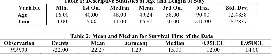
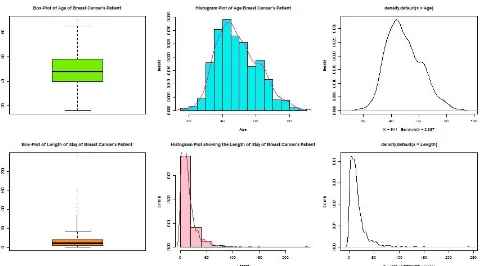
Table 1 shows the basic summary of age of the patients and their length of stay, it can be deduced that the average age of the patients with Breast Cancer is approximately 49 years old but while the average length of stay is 16 days. Figure 3 show the box-plot, histogram and density plot of Age and Length of stay of the patients. The box-plot revealed a presence of outliers in age and length of stay of patients but was much in Length of stay and this implies that the mean of time (Length) of stay (49.24 days) is not a true value to describe the whole data. The histogram shows the pattern of the data where it can have observed that the age of patients looks normally distributed while the histogram of length of stay skewed to left.
Table 1: Descriptive Statistics of Age and Length of Stay
Variable Min. 1st Qu. Median Mean 3rd Qu. Max. Std. Dev.
Age 16.00 40.00 48.00 49.24 58.00 90.00 12.4858
Time 1.00 5.00 11.00 15.81 20.00 240.00 18.2837
Table 2: Mean and Median for Survival Time of the Data
Observation Events Mean se(mean) Median 0.95LCL 0.95UCL
Figure 1: Multiple Bar Chart Showing the Distribution of Patients Diagnosed for Breast Cancer by Gender
Figure 2: Multiple Bar Chart Showing the Distribution of Patients Diagnosed for Breast Cancer by Status
Figure 3: Histogram, Density Plot and Box-Plot of Age and Length of Stay
0 20 40 60 80 100 120 140
2007 2008 2009 2010 2011 2012 2013 2014 2015 2016
Fre
q
u
en
cy
Years
Multiple Bar Chart Showing the Distribution of
Patients with Breast Cancer per Gender
Male
Female
0 20 40 60 80 100 120
2007 2008 2009 2010 2011 2012 2013 2014 2015 2016
Dead 34 20 22 15 17 3 22 20 16 48
Alive 28 83 93 38 85 64 117 100 55 61
Fre
q
u
en
cy
Year
Multiple Bar Chart Showing the Distribution of
Patients with Breast Cancer by Status
Dead
From the above, It can be deduced that out of the (939) patients admitted between years 2007-2016, 722 survived after the treatment, the mean value indicates that the mean time for patients to survive after the treatment is 22.27 and the median survival time (the time at which 50% of the subjects have reached the event is 13.00.
Kaplan-Meier Estimate of the Survival Function
Figure 4: Kaplan-Meier Estimate of the Survival Function
The above curve shows the survival plot of the whole data where it can be deduced that the probabilities of surviving is decreasing as time is progressing, the dashed lines are the upper and lower confidence intervals.
Estimation of Mean and Median of Survival Rate of the Data by Gender
Table 3: Mean and Median for Survival Time by Sex
Gender Observation Events Mean se(mean) Median 0.95LCL 0.95UCL
Male 32 26 24.8 7.71 15 12 32
Female 907 696 21.9 1.10 13 12 14
From the above table, it can be deduced that out of the 722 patients that survived the helmet 26 are male while 696 are female. The mean time for male patients to survive after the treatment is 24.8 days while that of female is 21.90 days. The median survival time (the time at which 50% of the subjects have reached the event) is 15 days for male and 13 days for female. This implies that female response to treatment faster than male patients.
Table 4: Survival Function of Male Patients
Time n.risk n.event survival std. error lower
95% CI
upper 95% CI
1 32 3 0.9062 0.0515 0.8107 1.000
3 28 2 0.8415 0.0651 0.7232 0.979
4 26 1 0.8092 0.0702 0.6827 0.959
5 25 1 0.7768 0.0744 0.6438 0.937
6 24 1 0.7444 0.0781 0.6061 0.914
9 22 1 0.7106 0.0815 0.5675 0.890
12 20 2 0.6395 0.0875 0.4891 0.836
13 18 2 0.5685 0.0911 0.4153 0.778
15 16 3 0.4619 0.0925 0.3120 0.684
16 13 3 0.3553 0.0893 0.2171 0.581
20 10 1 0.3198 0.0871 0.1874 0.546
21 9 1 0.2842 0.0844 0.1588 0.509
24 8 1 0.2487 0.0810 0.1314 0.471
31 7 1 0.2132 0.0768 0.1052 0.432
32 6 1 0.1776 0.0718 0.0805 0.392
33 5 1 0.1421 0.0656 0.0575 0.351
Table 5: Survival Function of Female Patients
time n.risk n.event survival std. error lower
95% CI
upper 95% CI
1 907 71 0.92172 0.00892 0.904404 0.9394
2 818 37 0.88003 0.01083 0.859049 0.9015
3 771 22 0.85492 0.01177 0.832151 0.8783
4 739 27 0.82368 0.01279 0.799000 0.8491
5 695 27 0.79168 0.01369 0.765297 0.8190
6 657 28 0.75794 0.01452 0.730017 0.7869
7 626 21 0.73252 0.01505 0.703599 0.7626
8 597 33 0.69203 0.01579 0.661768 0.7237
9 550 31 0.65302 0.01638 0.621699 0.6859
10 515 35 0.60864 0.01689 0.576412 0.6427
11 471 37 0.56083 0.01730 0.527926 0.5958
12 426 25 0.52792 0.01749 0.494722 0.5633
13 395 23 0.49718 0.01761 0.463835 0.5329
14 371 28 0.45965 0.01765 0.426330 0.4956
15 338 26 0.42430 0.01760 0.391162 0.4602
16 306 21 0.39518 0.01750 0.362319 0.4310
17 282 22 0.36435 0.01733 0.331921 0.3999
18 258 8 0.35305 0.01724 0.320819 0.3885
19 248 14 0.33312 0.01707 0.301281 0.3683
20 231 11 0.31726 0.01692 0.285773 0.3522
21 217 16 0.29386 0.01665 0.262977 0.3284
22 196 7 0.28337 0.01652 0.252770 0.3177
23 189 16 0.25938 0.01617 0.229540 0.2931
24 165 2 0.25624 0.01613 0.226494 0.2899
25 158 10 0.24002 0.01590 0.210787 0.2733
26 145 12 0.22016 0.01559 0.191630 0.2529
27 133 2 0.21685 0.01553 0.188450 0.2495
28 129 4 0.21012 0.01541 0.181995 0.2426
29 125 4 0.20340 0.01528 0.175557 0.2357
30 120 2 0.20001 0.01521 0.172315 0.2321
31 118 7 0.18814 0.01495 0.161005 0.2199
32 110 4 0.18130 0.01479 0.154504 0.2127
33 100 5 0.17224 0.01460 0.145872 0.2034
34 94 4 0.16491 0.01443 0.138915 0.1958
35 87 1 0.16301 0.01439 0.137114 0.1938
36 83 1 0.16105 0.01435 0.135242 0.1918
37 80 5 0.15098 0.01414 0.125661 0.1814
38 75 1 0.14897 0.01409 0.123754 0.1793
39 74 1 0.14696 0.01405 0.121849 0.1772
41 70 1 0.14486 0.01400 0.119855 0.1751
42 68 1 0.14273 0.01396 0.117831 0.1729
43 67 2 0.13847 0.01386 0.113795 0.1685
44 62 1 0.13623 0.01382 0.111672 0.1662
45 58 4 0.12684 0.01364 0.102733 0.1566
46 53 2 0.12205 0.01354 0.098202 0.1517
47 50 2 0.11717 0.01343 0.093594 0.1467
48 48 1 0.11473 0.01337 0.091300 0.1442
49 46 1 0.11223 0.01331 0.088956 0.1416
50 45 1 0.10974 0.01325 0.086620 0.1390
51 44 1 0.10725 0.01318 0.084292 0.1364
54 37 3 0.09855 0.01303 0.076052 0.1277
55 33 2 0.09258 0.01291 0.070442 0.1217
56 31 1 0.08959 0.01283 0.067663 0.1186
57 28 1 0.08639 0.01277 0.064668 0.1154
60 27 1 0.08319 0.01269 0.061696 0.1122
61 24 1 0.07973 0.01262 0.058454 0.1087
64 23 1 0.07626 0.01254 0.055246 0.1053
65 22 1 0.07279 0.01244 0.052072 0.1018
time n.risk n.event survival std. error lower 95% CI
upper 95% CI
67 19 1 0.06551 0.01222 0.045458 0.0944
73 17 1 0.06166 0.01209 0.041986 0.0906
74 16 1 0.05781 0.01193 0.038571 0.0866
76 15 2 0.05010 0.01152 0.031923 0.0786
81 12 2 0.04175 0.01101 0.024899 0.0700
82 9 1 0.03711 0.01072 0.021069 0.0654
84 8 1 0.03247 0.01033 0.017402 0.0606
93 7 1 0.02783 0.00984 0.013915 0.0557
105 6 1 0.02319 0.00923 0.010631 0.0506
114 5 1 0.01855 0.00847 0.007583 0.0454
132 4 2 0.00928 0.00628 0.002461 0.0350
150 2 1 0.00464 0.00454 0.000681 0.0316
240 1 1 0.00000 NaN NA NA
Figure 5: Kaplan Meier Estimate of the Survival Function by Gender
Table 6: Mean and Median for Survival Time by Age Interval Age
Interval
Observation events Mean se(mean) median 0.95LCL 0.95UCL
10-19 4 4 9.5 3.75 9.5 2 NA
20-29 23 22 21.7 4.62 19.0 4 32
30-39 185 138 19.7 1.52 14.0 13 16
40-41 294 241 19.1 1.31 11.0 10 14
50-51 217 163 18.7 1.32 14.0 12 16
60-61 149 109 22.8 2.12 15.0 12 18
70-71 53 35 25.1 3.94 14.0 11 28
80-81 11 10 11.5 3.30 8.0 3 NA
90-91 3 0 74.0 0.00 NA NA NA
Figure 6: Kaplan Meier Estimate of the Survival Function by Age Group
Cox Proportional Hazards Regression Analysis
Table 7: Cox Proportional Hazards Regression Analysis
Variable coef exp(coef) se(coef) z p-value
Age -0.006838 0.993186 0.003140 -2.177 0.0295
Sex -0.182796 0.832938 0.204328 -0.895 0.3710
Length -3.059215 0.046925 0.134172 -22.801 <2e-16
Year 0.005773 1.005789 0.014161 0.408 0.6835
Variable exp(coef) exp(-coef) lower .95 upper .95
Age 0.99319 1.0069 0.98709 0.99932
Sex 0.83294 1.2006 0.55807 1.24319
Length 0.04692 21.3108 0.03607 0.06104
Year 1.00579 0.9942 0.97826 1.03410
Concordance 0.993 Std. Error 0.01
Rsquare 0.991 Max Possible 1
Likelihood ratio test 4446 on 4 df p-value 0.000
Wald test 523.4 on 4 df p-value 0.000
Score (logrank) test 415.7 on 4 df p-value 0.000
From the above table, the column marked “z” gives the Wald statistic value. It corresponds to the ratio of each regression coefficient to its standard error. It shows that Age and Length have highly statistically significant coefficients. It means that the risk of death is higher in Year with a positive value while the risk of death is low in variable Age, Sex, and Length spent in hospital with negative value of coefficient. The p-value for Age is 0.0295, with a hazard ratio HR of 0.993186, indicating a strong relationship between the patients’ Age and patients risk of death and also the p-value and hazard ratio show a strong relationship between the time spent in the hospital and decreased risk of death. The beta coefficient for sex gives -0.1828 indicates that female patients have lower risk of death (lower survival rates) than male patients. It also shows that the hazard ratio is 0.832338. The p-value for all three overall tests (likelihood, Wald, and score) are less than 0.05, the test statistics are in close agreement, and the omnibus null hypothesis is soundly rejected therefore the model is significant.
The Log Rank Test
Table 8: Log Rank Test for Status of the Patient
d.f p-value Remark
Log Rank Test 0.000 1 0.900 Not Significant
Table 9: Log Rank Test for Sex of the Patient
d.f p-value Remark
From the tables above, since the p-value is greater than 0.05 across the gender but less than across the status, this implies that there is no statistically difference in the survival rates between males and females but there is statistically differences in the survival rates between dead and alive.
Wilcoxon test
Table 10: Goodness of Fit with Chi-Square Using Wilcoxon Test
Variable N Observed Expected (O-E)^2/E (O-E)^2/V d.f p-value Remark
Male 32 14.4 15.8 0.12058 0.189 0.20
0 1 0.700 Not Significant
Female 909 411.0 409.6 0.00465 0.189
Dead 217 0.00 102 102.1 203
203 1 0.000 Significant
Alive 724 425 409.6 0.00465 203
Both Wilcoxon and Log Rank Test gave the same decision but there is difference in their p-value with p-value of Wilcoxon Test lesser than Log Rank Test.
CONCLUSION
The results of various data analysis showed that the median survival time until the event occurs is 15 days for male and 13 days for female. Kaplan-Meier Estimator shows that female response to treatment faster than male patients with the mean time of 24.8 days and t = 21.90 days respectively, the survival plot shows that the probabilities of surviving is decreasing as time progresses, it also revealed that in all age groups, there is a decrease in their chance of surviving. The result of cox proportional hazard regression analysis shows that Age and Length have high statistical significant coefficients which means that the risk of death is higher in Year with a positive value while the risk of death is low in Age, Sex, and Length spent in hospital with negative value of coefficient. The Hazard Ratio (HR) of 0.993186, indicates a strong relationship between the patients’ Age and patients risk of death and between the time spent in the hospital and decrease risk of death. The beta coefficient for sex gives -0.1828 indicates that female patients have lower risk of death than male patients and the hazard ratio gives 0.832338. The Wilcoxon test and Long rank test revealed that there are no statistically differences in the survival rates between males and females but there is a statistically differences in the survival rates between Dead and Alive. It also shows that female patients have lower risk of death than male patients with the beta coefficient of -0.1828 while hazard ratio gives 0.832338.
REFERENCES
[AA00] Adebamowo C. A., Ajayi O. O. - Breast cancer in Nigeria. West Afr J Med.;19:179–191. 2000.
[ACS05] American Cancer Society - Breast Cancer Facts & Figures 2005–2006. American Cancer Society Inc. Atlanta 2005.
[A+06] Anderson B. O., Shyyan R., Eniu A., Smith R. A., Yip C. H., Bese N. S., Chow L. W., Masood S., Ramsey S. D., Carlson R.W. - Breast cancer in limited-resource countries: An overview of the Breast Health Global Initiative 2005 Guidelines. Breast J, 12(Suppl 1):S3-15. 2006.
[A+15] Akinde O. R., Phillips A. A., Oguntunde O. A., Afolayan O. M. - Cancer mortality pattern in Lagos University teaching hospital, Lagos, Nigeria. J Cancer Epidemiol. 2015.
[C+02] Chong P. N., Krishnan M., Hong C. Y., Swash T. S. - Knowledge and practice of breast cancer screening amongst public health nurses in Singapore. Singapore Med J, 43:509-516. 2002. http://www.biomedcentral.com/sfx_links.asp?ui =1471-2458-7-96&bibl=B12
[F+12] Ferlay J., Soerjomataram I., Ervik M., Dikshit R., Eser S., Mathers C. et al. - Globocan 2012: Estimated cancer incidence, mortality and prevalence worldwide in 2012. World Health Organization. 2012.
[G+06] Groot M. T., Baltussen R., Uyl-de Groot C. A., Anderson B. O., Hortobágyi G. N. - Costs and health effects of breast cancer interventions in epidemiologically different regions of Africa, North America, and Asia. Breast J , 12(Suppl 1):S81-90. 2006.
[J+06] Jemal A., Siege R., Ward E., Murray T., Xu J., Smigal C., Thun M. J. - Cancer statistics 2006. CA: A Cancer J Clin 2005, 56(2):106-130.
[J+10] Jemal A., Center M. M., DeSantis C., Ward E. M. - Global patterns of cancer incidence and mortality rates and trends. Cancer Epidemiol Biomarkers Prev. 2010; 19: 1893-1907.
[J+12] Jemal A., Bray F., Forman D., O’brien M., Ferlay J., Center M. et al. - Cancer burden in Africa and opportunities for prevention. Cancer. 2012; 118: 4372-4384.
[L+04] Lee E. O., Ahn S. H., You C., Lee D. S., Han W., Choe K. J., Noh D. Y. - Determining the main risk factors and high-risk groups of breast cancer using a predictive model for breast cancer risk assessment in South Korea. Cancer Nurs.;27(5):400-6. 2004.
[Myl17] Mylan B. - Cooperation in Cancer Cells. 2017.
[M+08] Mohammed A., Edino S., Ochicha O., Gwarzo A., Samaila A. A. - Cancer in Nigeria: a 10-year analysis of the Kano cancer registry. Niger J Med. 2008; 17: 280-284.
[P+05] Parkin D. M., Bray F., Ferlay J., Pisani P. - Global cancer statistics 2002. CA Cancer J Clin. 2005; 55:74–108.
[SW16] Stewart B., Wild C. P. - World Cancer Report 2014. Int Agency Res Cancer. 2016.
[S+01] Sadler G. R., Dhanjal S. K., Shah N. B., Shah R. B., Ko C., Anghel M., Harshburger R. - Asian India women: knowledge, attitudes and behaviors toward breast cancer early detection. Public Health Nurs.;18(5):357-63. 2001.