https://doi.org/10.5194/wes-3-845-2018
© Author(s) 2018. This work is distributed under the Creative Commons Attribution 4.0 License.
Assessing variability of wind speed: comparison and
validation of 27 methodologies
Joseph C. Y. Lee1,2, M. Jason Fields1, and Julie K. Lundquist1,2 1National Renewable Energy Laboratory, Golden, CO 80401, USA
2Department of Atmospheric and Oceanic Sciences, University of Colorado Boulder, Boulder, CO 80309, USA
Correspondence:Joseph C. Y. Lee ([email protected])
Received: 12 June 2018 – Discussion started: 30 July 2018
Revised: 4 October 2018 – Accepted: 16 October 2018 – Published: 5 November 2018
Abstract. Because wind resources vary from year to year, the intermonthly and interannual variability (IAV) of wind speed is a key component of the overall uncertainty in the wind resource assessment process, thereby creating challenges for wind farm operators and owners. We present a critical assessment of several common ap-proaches for calculating variability by applying each of the methods to the same 37-year monthly wind-speed and energy-production time series to highlight the differences between these methods. We then assess the accuracy of the variability calculations by correlating the wind-speed variability estimates to the variabilities of actual wind farm energy production. We recommend the robust coefficient of variation (RCoV) for systematically estimating variability, and we underscore its advantages as well as the importance of using a statistically robust and resistant method. Using normalized spread metrics, including RCoV, high variability of monthly mean wind speeds at a location effectively denotes strong fluctuations of monthly total energy generation, and vice versa. Meanwhile, the wind-speed IAVs computed with annual-mean data fail to adequately represent energy-production IAVs of wind farms. Finally, we find that estimates of energy-generation variability require 10±3 years of monthly mean wind-speed records to achieve a 90 % statistical confidence. This paper also provides guidance on the spatial distribution of wind-speed RCoV.
1 Introduction
The P50, a widely used parameter in the wind-energy indus-try, is an estimate of the threshold of annual energy produc-tion of a wind farm that the facility is expected to exceed 50 % of the time (Clifton et al., 2016). The P50 is usually estimated to apply over the lifetime of a wind farm, typi-cally 20 years. To estimate P50 in the wind resource assess-ment process, a single percentage value is usually assigned to represent the uncertainty for the desired time period at a wind site (Brower, 2012). The interannual variability (IAV) of wind resources, along with site measurements and wind-power-plant performance, is an important component of the overall uncertainty in power production (Clifton et al., 2016; Klink, 2002; Lackner et al., 2008; Pryor et al., 2006). The IAV is also incorporated in the measure–correlate–predict process (Lackner et al., 2008), which usually considers wind measurements spanning less than 2 years.
Analysts and researchers use numerous metrics to quantify wind-speed variability, and the most common method is stan-dard deviation (σ). For instance, the variability in historical or future wind resources is often represented as theσ from the annual-mean wind speed of a certain location (Brower, 2012). As wind turbine power generation is a function of wind speed, the variability of wind resources has important implications for the resultant long-term energy production. Financially, when the wind resource is projected to fluctuate more from year to year (Hdidouan and Staffell, 2017), the levelized cost of wind energy increases as well.
capacity factor. Lee et al. (2018) assess the spatial discrep-ancies between wind-speed variabilities of different tempo-ral scales, from hourly mean to annual-mean data. Bett et al. (2013) useσ and Weibull parameters to assess the wind variability in Europe. Extreme event analysis also offers an-other perspective to assess variability. For example, Cannon et al. (2015) examine extreme wind-energy generation events via reanalysis data and discuss the associated seasonal and IAV qualitatively. Leahy and McKeogh (2013) also quantify the return periods of multiweek wind droughts.
To quantify variability, the normalizedσor the coefficient of variation (CoV), the σ divided by the mean of a time series, is a commonly used tool. Justus et al. (1979) cal-culate and compare the CoVs of monthly and annual wind speeds at different sites across the United States. Baker et al. (1990) quantify interannual and interseasonal variations of both wind speed and energy production at three loca-tions in the Pacific Northwest. They find the annual CoVs ranged from 4 % to 10 %, matching the conclusions from Justus et al. (1979). Recently, Li et al. (2010) calculate hub-height wind-speed variance andσ over 30 years to spatially evaluate seasonal and IAV in the Great Lakes region. Bo-dini et al. (2016) estimate the IAV of wind resources with a modified version of CoV, using observed meteorological data in Canada. As the sample period increases, the IAVs of most sites gradually increase, averaging 5 % to 6 % among the chosen sites (Bodini et al., 2016). Krakauer and Co-han (2017) correlate the CoVs of monthly mean wind speeds with different climate oscillation indices and find the global mean CoV at 8 %. In addition to characterizing wind speed, the metric is also used to evaluate the benefits of grid inte-gration. For example, Rose and Apt (2015) conclude that the interannual CoV of aggregate wind-energy generation in the central United States is 3±0.1 %, much smaller than that of individual wind plants, which varies between 5.4 % and 12 %,±4.2 %.
Aside from CoV, other metrics representing the spread of data have also been chosen to estimate variability in the literature. For example, the robust coefficient of variation (RCoV) normalizes the median absolute deviation (MAD) with the median. Gunturu and Schlosser (2012) quantify the spatial RCoV of wind-power density in the United States and demonstrate that the regions east of the Rockies, es-pecially the Plains, generally have weaker variability and higher availability of wind resources. The seasonality index, originally used in Walsh and Lawler (1981) for precipitation purposes, is another measure to express variability. The sea-sonality index is defined as the sum of the absolute deviations of monthly averages from the annual mean, normalized with the annual mean. Chen et al. (2013) use the seasonality in-dex to assess the interannual trend and the variability of wind speed in China, and they relate wind-speed IAVs to climate oscillations.
Alternative variability metrics emphasize the long-term trends via contrasting wind speeds of different periods. The
“wind index”, used in Pryor et al. (2006) and Pryor and Barthelmie (2010), is a ratio of wind speeds of a reference period and an analysis period. An entirely different wind in-dex evaluated in Watson et al. (2015) is a ratio of spatially averaged wind speeds during two different periods.
Despite the importance of long-term variability, the wind-energy industry lacks a systematic method to quantify this uncertainty. As various metrics to assess variability exist, a comprehensive comparison of measures is necessary. There-fore, the goal of this study is to evaluate various methods of estimating intermonthly and IAV in a reliable way us-ing a long-term, consistent database. Specifically, our objec-tive is to determine an optimal metric or metrics for relat-ing wind-speed variability to energy-production variability. We describe the wind-speed and energy-generation data, the methodology, and the chosen variability metrics in Sect. 2. We evaluate different variability measures via two case stud-ies in Sect. 3. We also contrast the results computed from monthly mean and annual-mean data, and we illustrate the spatial distribution of wind-speed variability in Sect. 3. We then recommend the best practice in using the ideal method in Sect. 4. We focus on the applicability of imposing such metrics to quantify the variabilities of wind speeds and wind-energy production.
2 Data and methodology
2.1 Wind and energy data
In this study, we use a 37-year time series of monthly mean wind speed and monthly total wind-energy production in the contiguous United States (CONUS). For wind speed, we use hourly horizontal wind components in the National At-mospheric and Space Administration’s Modern-Era Retro-spective Analysis for Research and Applications, Version 2 (MERRA-2), reanalysis data set (Gelaro et al., 2017; GMAO, 2015) from 1980 to 2016. We use these components to de-rive the monthly mean wind speed at 80 m above the surface, which represents hub height in this study, via the power law (Eq. 1) and the hypsometric equation (Eq. 2):
u(z2)
u(z1)
=
z2
z1
α
, (1)
z2−z1=RdTln
p
2
p1
. (2)
In Eq. (1),u(z1) andu(z2) are the horizontal wind speeds, at heightsz1andz2, in which wind speeds are the square root of the sum of squared horizontal wind components, andαis the shear exponent. In Eq. (2),Rdis the dry air gas constant,
T is the average temperature between levels z1 andz2, and
at 850 or 500 hPa may be closer to 80 than 10 m above the surface; in that case, we use data at the next available level of 850 or 500 hPa to derive the heights of that level and thus to extrapolate the wind speed at 80 m.
The horizontal resolution of the MERRA-2 is 0.5◦in lat-itude (about 56 km) and 0.625◦in longitude (about 53 km). The MERRA-2 reanalysis interpolates the data and the meta-data at the exact output latitude and longitude; hence the wind speed, air density, and elevation refer to the grid points with the particular sets of latitude and longitude (Bosilovich et al., 2016). Thus, the longest distance between a wind farm and the closest MERRA-2 grid-cell center is about 39 km.
For energy-production data, we use the net monthly energy production of wind farms in megawatt hours (MWh) from the US Energy Information Administration (EIA) between 2003 and 2016. Each of the wind farms has a unique EIA identifi-cation number. After we leave out about 300 wind sites with incomplete or substantially zero production data, a total of 607 wind farms in the CONUS are selected for this analy-sis. For simplicity, the CONUS in this analysis is defined as the area bounded by 127◦W, 65◦W, 24◦N, and 50◦N, and geographically includes the 48 states in CONUS and Wash-ington, D.C. (Fig. 1).
2.2 Methodology
2.2.1 Linear regression and data post-processing
We focus on the direct relationship between wind speed and energy production to investigate approaches for calculating long-term variability. Therefore, we must minimize the in-fluence from other determinants of energy production, such as curtailment and maintenance. First, we eliminate data with zero values for monthly energy production, which is typical in the first months of a new wind farm. Next, we linearly regress the monthly total energy production on the monthly mean MERRA-2 80 m wind speed at the closest grid point to each wind farm from 2003 to 2016. In other words, each wind site is assigned its own regression equation. We then re-move any production data below the 90 % prediction interval to exclude underproduction for reasons other than low wind speeds, and omit the data above the 99 % prediction interval, or potentially erroneous overproduction. Prediction intervals are calculated via thet values and the standard error of pre-diction (Montgomery and Runger, 2014). In other words, we define the outliers of energy production using the threshold of 1.64 times below the standard error and 2.58 times above the standard error of the site-specific regression. We also ap-ply a third-order polynomial fit (Archer and Jacobson, 2013), and it leads to very similar results to the linear model. Hence, we focus on presenting the results from the linear fit in this study.
After regressing the outlier-free energy data on wind speed, we then filter the wind farms based on the coefficient of determination (R2), which indicates the confidence of the
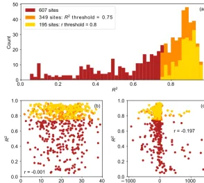
Figure 1.Wind farm locations in the CONUS: nonfiltered 607 sites in dark red,R2-filtered 349 sites in orange, andr-filtered 195 sites in yellow. The yellow square represents the Oregon site and the yel-low star indicates the Texas site (Table 2). The grey box illustrates the boundary of the CONUS used in this study.
linear regression. We select theR2threshold of 0.75: 349 of the original 607 wind farms pass this filter. Through this fil-ter, we ensure that wind speed is the primary driver of energy production in the wind farms with highR2values. Lunacek et al. (2018) also use a similarR2-filtering method with a threshold of 0.7. Considering some farms lack years of com-plete generation data, we extend the monthly energy produc-tion to 37 years using the same site-specific linear models with the monthly MERRA-2 wind speed. In other words, we compute any missing energy-production data from 1980 to 2016 based on the linear fit from the years that do exist in the data set. Herein, we refer to this long-term extension of data as the predicted energy production. Of the 349 wind farms, 7.5 years is the median of the energy data that are derived via the linear fit, given the available EIA records between 2003 and 2016.
We then further apply a second filter using the Pearson’s correlation coefficient (r) between the predicted and actual monthly energy production, and we only choose the 195 wind farms withrlarger than 0.8. As a result, of ther-filtered wind sites, we ensure wind speed is the primary driver of wind-power production, and we confirm the energy predic-tions match well with those observed.
The nonfiltered,R2-filtered, andr-filtered wind farms car-pet most of the popular wind farm regions across the CONUS (Fig. 1), even with the high r threshold of 0.8. Thus, the r-filtered samples provide a sufficient representation of the wind farms across the United States. To illustrate our anal-ysis with examples, we select one site in Oregon (OR) and another site in Texas (TX) that demonstrate distinct wind-speed distributions. We choose the two sites to contrast the results of different variability metrics throughout the paper; both sites pass therfilter (Fig. 1).
the closest MERRA-2 grid point and the actual wind farm, but we find no statistical relationship. In particular, horizon-tal and vertical discrepancies between the model and the ob-servations do not affect the resultantR2in the linear regres-sions. More than half of the 607 wind farms pass theR2 fil-ter, and more than half of those pass the r filter (Fig. 2a). Additionally, the correlation betweenR2and the horizontal distance between the closest MERRA-2 grid point and the actual wind farm is close to zero (Fig. 2b); the correlation betweenR2and the vertical difference between the modeled grid point and the actual wind site is also weak (Fig. 2c). In other words, the horizontal and vertical distances between the MERRA-2 grid points and the wind farms have no appar-ent impact on the represappar-entativeness of the wind farms in the linear regression.
Additionally, we analyze the uncertainty of the linear-regression method. We first test the influence of the error term in the regression, to account for the uncertainty asso-ciated with the input data. After a wind farm passes theR2 threshold of 0.75, we add a random value within 1 standard error to the predicted energy production of each month. This random error term introduces uncertainty to the regression process but does not affect theR2of the site-specific regres-sion. Furthermore, we also test the sensitivity of theR2and r thresholds by analyzing the results after modifying those limits. Specifically, we loosen theR2andrthresholds to 0.6 and 0.7, and we tighten theR2andrthresholds to 0.85 and 0.9. Loosening these thresholds increases the sample sizes of the wind farms that pass the filters and tightening the thresh-olds results in the opposite.
We test other factors that could undermine these regres-sions. We considered the hub-height air density extrapolated from MERRA-2 as another regressor in the regressions, but air density is a statistically insignificant predictor and thus is not discussed in the rest of this study. When we replace the prediction interval with the confidence interval, the sample sizes increase from 349 and 195 sites to 555 and 209 wind farms. However, at least 7 years of energy data are derived from the regression for 99 % of the samples, because confi-dence intervals are smaller than prediction intervals by def-inition. We also considered removing the long-term means and the impacts of annual cycles, yet the sample sizes de-crease to 121 and 69 locations, and the regression fills at least some of the energy data for more than 99 % of the sites. Finally, to ensure these results were not specific to the MERRA-2 data set, we perform the same analysis on the ERA-Interim reanalysis data set (Dee et al., 2011). The re-sults of the key variability parameters such as σ, CoV, and RCoV resemble the findings using MERRA-2; hence we fo-cus on the MERRA-2 findings in this study.
Our analysis, although comprehensive, is constrained by the quality of our data. On the one hand, reanalysis data sets have errors and biases in wind-speed predictions from complexities in elevation and surface roughness (Rose and Apt, 2016). Reanalysis data sets also demonstrate long-term
trends of surface wind speeds (Torralba et al., 2017). The MERRA-2 data set can also depict different meteorologi-cal environments than those at the wind farm locations, es-pecially in complex terrain. The MERRA-2 data of coarse temporal and spatial resolutions may also represent a lower intermonthly or IAV than the wind sites actually experi-ence. Thus, regressing actual energy production on reanaly-sis wind speed adds uncertainty to our analyreanaly-sis. On the other hand, constrained by the monthly total energy-production data from the EIA, our analysis ignores the signals finer than monthly cycles. The quality of the EIA data also varies across wind sites; therefore the filtering process via linear regression is necessary.
2.2.2 Variability metrics relating wind speeds and energy production
To evaluate the variabilities of both the wind speeds and the predicted energy generation from the filtered wind farms, we investigate a total of 27 combinations and variations of ex-isting methods describing the spread of data. We categorize different variability metrics according to statistical robust-ness (insensitivity to assumptions about the data; for exam-ple, Gaussian distribution) and statistical resistance (insensi-tivity to outliers) (Wilks, 2011). Of the 27 variability meth-ods tested, we select four representative measures to perform a comparison and discuss in detail, according to their robust-ness, resistance, and the nature of normalization by an aver-age metric:
1. RCoV, defined as the MAD divided by the median (Gunturu and Schlosser, 2012; Watson, 2014), is a spread metric divided by an average metric and is both statistically robust and resistant.
2. Range (maximum minus minimum) divided by trimean (weighted average among quartiles) is a spread metric normalized by an average metric, and the numerator is not resistant.
3. CoV (Baker et al., 1990; Bodini et al., 2016; Hdidouan and Staffell, 2017; Krakauer and Cohan, 2017; Rose and Apt, 2015; Wan, 2004), defined as theσdivided by the mean, is a spread metric normalized by an average met-ric, and neither the denominator nor the numerator are robust or resistant.
4. σis simply a spread metric that is not robust or resistant.
0.0 0.2 0.4 0.6 0.8 1.0
R2
0 10 20 30 40 50
Count
(a) 607 sites
349 sit es: R2 t hreshold = 0.75
195 sites: r threshold = 0.8
0 10 20 30 40
Horizontal distance (km) 0.0
0.2 0.4 0.6 0.8 1.0
R
2
r = -0.001
(b)
1000 0 1000
Elevation difference (m) 0.0
0.2 0.4 0.6 0.8 1.0
R
2
r = -0.197 (c)
Figure 2.(a)Histogram ofR2of all nonfiltered sites (dark red),R2-filtered sites (orange), andr-filtered sites (yellow);(b)scatterplot of theR2and the horizontal distance between the closest MERRA-2 grid cell and the actual locations of the sites using the same color scheme in(a);(c)scatterplot of theR2and the elevation difference between the closest MERRA-2 grid cell and the actual locations of the wind sites using the same color scheme in(a). Therin(b)and(c)represents the Pearson’srusing all nonfiltered sites.
developed by Bandi and Apt (2016), we also analyze the re-sults from the exponential CoV and the exponential RCoV in this paper (Table B1).
In addition to calculating variabilities with the spread mea-sures, we evaluate other diagnostics that describe distribution characteristics. These diagnostics include averaging metrics, such as the arithmetic mean (not resistant) and median (the 50th percentile, which is resistant); symmetry metrics, such as skewness (involving the third moment, not robust or resis-tant) and the Yule–Kendall Index (YKI, robust and resisresis-tant); a tailedness metric, namely kurtosis (involving the fourth moment, not robust or resistant); the Weibull scale and shape parameters (not robust); and the autocorrelation with a 1-year lag to dissect the interannual cycles. We summarize the diag-nostics evaluated in this analysis in Table B2. Along with the regression results, results from the four representative vari-ability metrics and other distribution diagnostics demonstrate differences between the two selected sites (Table 2).
Herein, we quantify the variabilities of the 37-year ex-tended time series of wind speed and energy production via different methods, using a range of time frames: 1 year, 2 years, and up to 37 years for each wind farm. A metric is considered useful when the resultant wind-speed variabil-ity correlates well with the resultant energy-production vari-ability across wind farms, even when random errors are
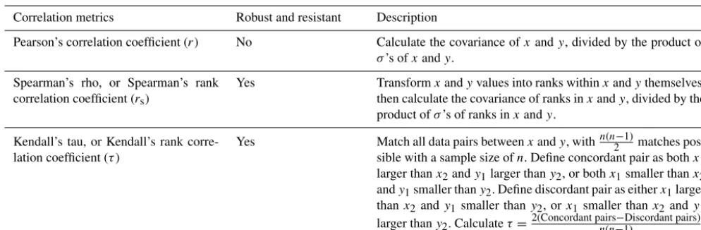
im-plemented and the thresholdsR2andrare changed. In this analysis, we compare results with three correlation metrics: Pearson’sr, Spearman’s rank correlation coefficient (rs), and Kendall’s rank correlation coefficient (τ) (Table 1).
Table 1.Details of the three correlation metrics applied, adapted from Wilks (2011). All three metrics yield values between−1 and 1.
Correlation metrics Robust and resistant Description
Pearson’s correlation coefficient (r) No Calculate the covariance ofxandy, divided by the product of
σ’s ofxandy.
Spearman’s rho, or Spearman’s rank correlation coefficient (rs)
Yes Transformxandyvalues into ranks withinxandythemselves,
then calculate the covariance of ranks inxandy, divided by the product ofσ’s of ranks inxandy.
Kendall’s tau, or Kendall’s rank corre-lation coefficient (τ)
Yes Match all data pairs betweenxandy, withn(n2−1)matches
pos-sible with a sample size ofn. Define concordant pair as bothx1
larger thanx2andy1larger thany2, or bothx1smaller thanx2
andy1smaller thany2. Define discordant pair as eitherx1larger
thanx2andy1smaller thany2, orx1smaller thanx2andy1
larger thany2. Calculateτ=2(Concordant pairsn(n−−1)Discordant pairs).
To relate the IAVs between wind speed and energy pro-duction, we also perform the same analysis for annual-mean data. Strictly speaking, calculating the variabilities using monthly mean data yields intermonthly variabilities, because the results account for monthly, seasonal, and annual signals. To isolate the signals from interannual variations, we also ex-amine the metrics and their correlations between the annual means of hub-height wind speeds and energy production, af-ter linear regressing and filaf-tering via monthly data. However, the samples from each site are then limited to 37 data points of annual wind speed and energy production. Besides, select-ing de-trended data from long-term means to calculate vari-abilities and their correlations leads to trivial results because of the small sample sizes and hence is omitted in this study.
2.2.3 Investigation of wind-speed RCoV
After we demonstrate that RCoV is the most systematic ap-proach in linking wind-speed and energy-generation vari-abilities in Sect. 3.2, we further examine the details of us-ing RCoV, specifically determinus-ing the minimum length of wind-speed data necessary to quantify variability effectively. We use 37 years of wind speed in every MERRA-2 grid cell in the CONUS (a total of 5049 grid points), and we calcu-late the RCoVs with 1 to 37 years of data for each grid cell. Because the RCoVs calculated using data between 1980 and 2016 are only samples of the true long-term wind-speed vari-ability and hence the results involve uncertainty, we select a confidence interval approach.
We assume that the distribution of RCoV is Gaussian with infinite years of wind speed. Hence, we use a chi-square (χ2) distribution to set bounds for theσ’s from samples of RCoV. In other words, because the derived RCoVs differ with the years of wind speeds sampled, we use theχ2distribution to quantify the confidence intervals of RCoV for each sample size. To determine the minimum data required for RCoV cal-culation, we use the following criterion (Montgomery and
Runger, 2014):
σ37≥
v u u t
(ni−1)σi2
χα/2,n2
i−1
, (3)
whereσ37 is the predetermined 37-yearσ of RCoV; ni is the sample size ofnyears in yeari, which is between 1 and 36 years;σi2is the variance of the sample of RCoVs in yeari; andχα/2,n2
i−1is the percentage point of theχ
2distribution given the confidence level ofαand the degrees of freedom ofni−1. We select a pair ofαlevels, 90 % and 95 %; hence we use four percentage points of theχ2distribution at 0.025, 0.05, 0.95, and 0.975 to construct the respective confidence intervals. Because the 37-year RCoV is an estimate of the truth, which is the wind-speed RCoV of infinite years, its singular value does not yield any variance or possess any dis-tribution shape. Thus, to construct the confidence interval of theσ of the truth, we set the predeterminedσ37as a fraction of the 37-year RCoV. Particularly, theσ37’s are 10 % and 5 % of the 37-year RCoV for the 90 % and 95 % confidence lev-els, respectively.
Table 2.Site details, monthly means, and annual means of various metrics at the two selected sites based on 37 years of monthly and annual wind speeds, and 37 years of predicted and actual energy production; and the CONUS medians of wind-speed metrics using 37 years of monthly and annual-mean data.
Site specifics OR site TX site CONUS median
Location, region, and state Condon, Columbia Bryson, northwest of 5049 MERRA-2
Gorge, OR Fort Worth, TX grid points
Nominal capacity (MW) 24.6 120 –
Elevation at closest MERRA-2 grid point – elevation of actual wind farm (m)
−501.4 −67.4 – Horizontal distance between MERRA-2 location and actual
lo-cation (km)
33.07 21.22 –
R2of final linear regression 0.868 0.794 –
Root mean square error of final linear regression (MWh) 1140.5 4185.0 –
Pearson’srbetween predicted and actual energy 0.906 0.809 –
Variability metrics Monthly Annual Monthly Annual Monthly Annual
mean mean mean mean mean mean
37-year wind-speed RCoV 0.082 0.029 0.094 0.023 0.102 0.021
37-year energy-production RCoV 0.226 0.059 0.166 0.041 – –
Actual energy-production RCoV 0.233 0.067 0.212 0.055 – –
37-year wind-speed trimeanrange 0.893 0.129 0.596 0.122 2.066 1.316
37-year energy-productiontrimeanrange 2.050 0.288 1.059 0.218 – –
Actual energy-production trimeanrange 1.768 0.307 1.303 0.305 – –
37-year wind-speed CoV 0.134 0.036 0.127 0.031 0.143 0.031
37-year energy-production CoV 0.333 0.081 0.225 0.055 – –
Actual energy-production CoV 0.341 0.088 0.279 0.089 – –
37-year wind-speedσ 0.909 0.242 0.964 0.234 0.895 0.203
37-year energy-productionσ 2.599 0.632 5.828 1.421 – –
Actual energy-productionσ 2.663 0.687 6.964 2.228 – –
Other 37-year wind-speed diagnostics Monthly Annual Monthly Annual Monthly Annual
mean mean mean mean mean mean
Mean (m s−1) 6.79 6.79 7.59 7.59 6.45 6.45
Median (m s−1) 6.64 6.79 7.63 7.57 6.51 6.45
Kurtosis 0.886 −0.962 −0.663 −0.872 −0.482 −0.373
Skewness 0.811 −0.129 −0.074 0.172 0.045 0.061
YKI 0.153 0.101 −0.072 0.041 −0.024 0.023
12-month-lag autocorrelation 0.324 0.039 0.525 −0.052 0.578 0.023
3 Results
3.1 Case studies: Oregon and Texas sites
We select two sites from two different geographical re-gions with considerable wind-energy deployment, the south-ern Plains and the Pacific Northwest in the United States, to contrast the results of various variability metrics. Based on the site-specific regressions, we extend the monthly energy-production time series to 37 years (Fig. 3a and b) for the two sites. Both sites pass theR2filter at 0.75 and therfilter at 0.8. Although the OR site is farther from the closest MERRA-2 grid point in a region with more complex terrain, the resultant R2 (0.87) and predicted–actual-energy Pearson’s r (0.91) are larger than those of the TX site (0.79 and 0.81, respec-tively) (Table 2). The 37-year-average wind speed of about
7.6 m s−1at the TX site is larger than that of the OR site at about 6.8 m s−1(Table 2). Additionally, the 12-month-lag au-tocorrelations demonstrate that the annual cycle of monthly wind speeds of the TX site is stronger than that of the OR site, yet the autocorrelations of the sites, 0.53 and 0.32, are still lower than the CONUS median of 0.58 (Table 2).
wind-Figure 3.(a)Time series of MERRA-2 monthly mean 80 m wind speed (black), actual monthly net EIA energy production (lime), and extended monthly energy production from 1980 to 2016 based on linear regression (green) at the OR site;(b)time series at the TX site with the same annotations as in(a);(c)histograms of MERRA-2 monthly mean wind-speed distribution (black) and yearly mean wind-speed distribution (grey) at the OR site from 1980 to 2016. The blue curve indicates the Gaussian fit of the monthly mean wind speeds via the mean and theσ, and the cyan curve represents the Gaussian fit of the annual-mean data;(d)histograms and curves of the Gaussian fit of wind-speed distributions at the TX site with the same annotations as in(c).
speed distribution is very close to symmetric with fewer out-liers (Fig. 3d), which is supported by near-zero skewness and YKI (Table 2), only 64.6 % of monthly data fall within 1σ from its mean. For annual-mean wind speeds, the averaging with a 12-month time span at both sites reduces the ranges and thus leads to kurtosis close to −1 (Table 2). Although the skewness and YKI are close to 0 (Table 2), only 59.5 % and 56.8 % of the annual-mean wind speeds fall within 1σ from the means of the OR and TX sites, respectively.
The four selected variability methods yield similar re-sultant monthly variabilities that are close to the respec-tive CONUS medians based on the 37-year monthly data. For variabilities of monthly wind speeds, the differences be-tween the two sites are slight because the comparison among the results of the four metrics is inconclusive (Table 2): the monthly variabilities are not far from the national medians (Table 2). However, results from the normalized spread met-rics (RCoVs, range divided by trimean, and CoV) using the 37-year and the observed energy production illustrate that the OR site generates more variable wind power than the TX site (Table 2). The magnitudes of the variabilities between the 37-year and the actual monthly energy production are also comparable, and the discrepancies between them are larger at the TX site than the OR site. Nonetheless, the predicted and the observed monthly energy production of the two sites demonstrate similar variability characteristics overall.
Moreover, when we apply the four selected methods to the annual-mean data, the metrics describe IAV exactly. For both variables, wind speed and energy generation, nearly all
met-rics illustrate that the OR site has stronger IAV than the TX site, except for usingσ to quantify energy-production IAV (Table 2). Echoing the results of the monthly data mentioned previously, the use of normalized metrics suggests the energy production at the OR site varies more than that at the TX site, intermonthly and interannually. Note that all the IAVs are smaller than the variabilities calculated using monthly data (Table 2), because the annual averaging collapses variations in the data.
Additionally, the magnitudes of energy variabilities and IAVs are also nearly or more than twice as large as those of wind speed (Table 2). The reason is the nature of the power curve: wind-power generation is a function of wind speed cubed at wind speeds below rated. Therefore, small wind-speed variations propagate into large energy-production fluc-tuations that are discernible in monthly and yearly data.
3.2 Variability metrics comparisons
energy-0.050 0.075 0.100 0.125 0.150 0.175 Wind-speed RCoV 0.10 0.15 0.20 0.25 0.30 0.35 0.40 Energy-production RCoV (a)
r = 0.856
0.5 0.6 0.7 0.8 0.9
Wind-speed trim eanrange
1.0 1.5 2.0 2.5 E n e rg y -p ro d u ct io n ra n g e tr im e a n (b)
r = 0.635
0.100 0.125 0.150 0.175 0.200 0.225 Wind-speed CoV 0.15 0.20 0.25 0.30 0.35 0.40 0.45 0.50 Energy-production CoV (c)
r = 0.704
0.6 0.8 1.0 1.2 1.4 1.6
Wind-speed 0 5 10 15 20 25 30 E n e rg y -p ro d u ct io n (d)
r = 0.184
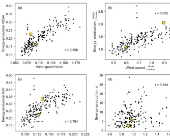
Figure 4.Scatterplots of 37-year wind-speed variability and energy variability via four metrics:(a)RCoV,(b) trimeanrange ,(c)CoV, and(d)σ, based on monthly data from the 195r-filtered wind sites. Each black dot represents each filtered site, and thervalue at the corner of each panel indicates the Pearson’srbetween each pair of wind-speed and energy-production spread metrics. The yellow square and the yellow star denote the OR and the TX sites, respectively.
generation variability, and vice versa (Fig. 4a). For instance, the moderate 37-year wind-speed RCoVs of the OR and TX sites indicate modest fluctuations in energy production be-tween months (Fig. 4a). On the other hand, a nonresistant method, range divided by trimean, leads to a lowerr (0.64) and suggests the OR site has variable wind speed and energy production (Fig. 4b). For the other two nonrobust and non-resistant methods, the CoV results in a modestr(0.70) with a similar scatter as the RCoV (Fig. 4c); the σ, not normal-ized by an average metric, does not relate wind-speed and energy variabilities effectively (Fig. 4d). The positions of the two wind farms relative to the rest of the sites in Fig. 4 il-lustrate that the TX site experiences average variabilities in wind resource and energy production, whereas the OR site has above-average energy-generation variability. Overall, the four methods lead to different representations of energy vari-ability at the OR site.
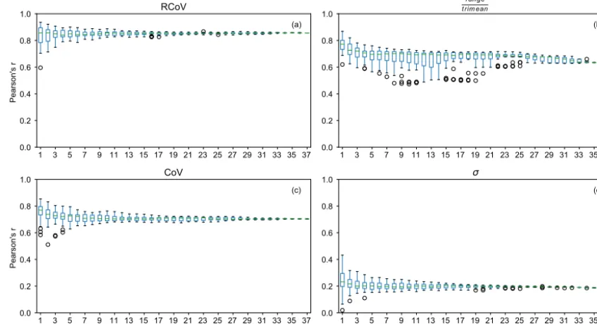
By increasing the years included in the variability cal-culations using monthly data, the resultant correlations of most metrics vary less, the correlations gradually converge to their 37-year values, and their asymptote periods vary. The 37-year Pearson’sr values from the four selected met-rics between wind-speed and energy-production variabilities in Fig. 4 transform into the 37-year marks in Fig. 5, and we use a 5 % threshold of normalized deviation to determine the asymptote periods. Particularly, ther’s from RCoV and CoV
(Fig. 5a and c) reach their respective asymptotes steadily with longer length of data, whereas ther’s from range di-vided by trimean do not (Fig. 5b). The 37-year correlation usingσ is weak and thus the method is not actually useful: while ther’s approach the 37-year benchmark (Fig. 5d), this correlation value is so low (0.2) as to be ineffective. Paired with a high long-termr, the asymptote period of a metric indicates the appropriate time span of wind-speed data re-quired to represent the variability of wind-energy production. For example, the resultantr’s using RCoV approach a high value after just 3 years, meaning one needs 3 years of wind-speed data to estimate the wind-wind-speed variability so as to ad-equately infer the energy-production variability of a certain or potential wind farm via RCoV.
1 3 5 7 9 11 13 15 17 19 21 23 25 27 29 31 33 35 37 0.0
0.2 0.4 0.6 0.8 1.0
Pearson's r
(a) RCoV
1 3 5 7 9 11 13 15 17 19 21 23 25 27 29 31 33 35 37
0.0 0.2 0.4 0.6 0.8 1.0
(b)
range t rim ean
1 3 5 7 9 11 13 15 17 19 21 23 25 27 29 31 33 35 37
Year 0.0
0.2 0.4 0.6 0.8 1.0
Pearson's r
(c) CoV
1 3 5 7 9 11 13 15 17 19 21 23 25 27 29 31 33 35 37
Year 0.0
0.2 0.4 0.6 0.8 1.0
(d)
Figure 5.Box plots of Pearson’s r between wind-speed variability and energy variability for different analysis time frames, from 1 to 37 years:(a)RCoV,(b) trimeanrange ,(c)CoV, and(d)σ, based on the monthly data from the 195r-filtered wind sites. Eachr represents the correlation using all the filtered sites of a particular time frame. The 37-year correlations are equal to thervalues listed in Fig. 4. The box and whiskers represent the third quartile plus the 1.5 times of interquartile range (IQR), the third quartile, the median, the first quartile, and the first quartile minus the 1.5 times of IQR.
the highestrs, and thersof RCoV is the second largest (Ta-ble 3). More importantly, the asymptote periods of RCoV are the smallest of all, regardless of the choice of correlation coefficient. In other words, fewer years of data are neces-sary to calculate RCoV to effectively relate wind-speed and energy variabilities than any other metric. Overall, when a spread metric yields strong correlations between variabilities of wind speed and energy generation, the correlation metrics agree with each other (Table 3). Therefore, the results in this paper focus on Pearson’sr, which is a commonly used cor-relation coefficient.
In addition to the spread metrics, other distribution diag-nostics also yield strong correlations between the 37-year monthly wind speed and energy production. For example, kurtosis and skewness result inrandrs above 0.9. Because we determine the asymptote periods based on normalized de-viations, when the 37-year correlation benchmark of a metric is high, the respective asymptote period tends to be shorter. Therefore, only 1 year of monthly data is required to com-pute kurtosis and skewness adequately, except for using rs in kurtosis, where thosers’s of the smaller number of years are low (Table 3). Moreover, the symmetry and the shape of the energy-production distribution can be characterized using wind-speed data, given the moderately strong correlations of YKI and the Weibull shape parameter (Table 3).
Additionally, we also perform the same correlation and asymptote analyses on the data from changing the R2 and
Table 3.Correlations and the associated asymptote periods of wind-speed variability and energy variability using various spread methods and distribution diagnostics with different correlation metrics, based on the monthly data of the 195r-filtered wind sites.
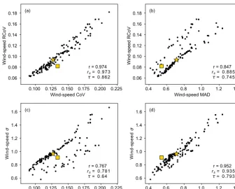
Spread metrics 37-year Asymptote years 37-year Asymptote years 37-year Asymptote years
r fromr rs fromrs τ fromτ
CoV 0.704 5 0.754 4 0.565 9
σ
median 0.743 4 0.781 3 0.595 4
σ
trimean 0.728 4 0.770 3 0.583 6
IQR
mean 0.818 4 0.821 3 0.636 6
IQR
median 0.845 3 0.843 3 0.662 6
IQR
trimean 0.834 3 0.834 3 0.650 6
RCoV 0.856 3 0.836 2 0.663 3
MAD
mean 0.834 3 0.822 3 0.648 5
MAD
trimean 0.848 3 0.832 3 0.660 5
Range
mean 0.609 30 0.711 28 0.516 31
Trimmedσ
median 0.806 3 0.807 3 0.631 5
Trimmedσ
trimean 0.794 4 0.801 4 0.622 6
Seasonality index, modified from Walsh and Lawler (1981)
0.744 5 0.766 4 0.584 7
Other diagnostics
Kurtosis 0.936 1 0.934 14 0.785 24
Skewness 0.943 1 0.938 1 0.798 18
YKI 0.778 23 0.712 33 0.538 34
Weibull shape parameter 0.721 4 0.741 5 0.559 7
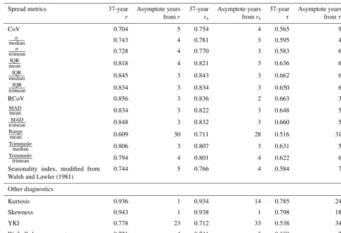
Further, normalized and simple spread metrics yield differ-ent relative wind-speed variabilities between wind sites. On the one hand, the correlations coefficients between 37-year monthly mean wind-speed RCoV and CoV, two spread met-rics that are normalized by average metmet-rics, are nearly unity (Fig. 6a). The comparison between two simple spread met-rics, MAD andσ, results in correlation coefficients close to 1 also (Fig. 6d). The relative positions of the OR site highlight the differences between Fig. 6a and d: compared to other wind farms, the OR site has moderate wind-speed RCoV and CoV, but small MAD andσ. Compared to Fig. 6a, the lower rs andτ in Fig. 6d illustrate that MAD andσ can misrepre-sent the relative wind-speed variabilities of a wind site. On the other hand, the results between a normalized spread met-ric (RCoV and CoV) and the respective simple spread metmet-ric (MAD and σ), which is also the numerator of the normal-ized spread metric, lead to weaker correlations (Fig. 6b and c). The r, rs, and τ between 37-year monthly wind-speed RCoV andσ are 0.684, 0.738, and 0.579, respectively (not shown). The wind sites with slower average wind speeds and thus disproportionately larger normalized spread results cause the deviations from perfect correlations in Fig. 6b and
c. Therefore, normalized spread metrics, which account for the differences in wind-speed magnitude, become advanta-geous over simple spread metrics in comparing variabilities of wind sites. Note that we demonstrate similar comparisons between wind-speed spread metrics via annual-mean data in Fig. A2 (Appendix A).
0.100 0.125 0.150 0.175 0.200 0.225 Wind-speed CoV
0.06 0.08 0.10 0.12 0.14 0.16 0.18
Wind-speed RCoV
(a)
r = 0.974
rs = 0.973 = 0.862
0.4 0.6 0.8 1.0 1.2 1.4
Wind-speed MAD 0.06
0.08 0.10 0.12 0.14 0.16 0.18
Wind-speed RCoV
(b)
r = 0.847
rs = 0.885 = 0.745
0.100 0.125 0.150 0.175 0.200 0.225 Wind-speed CoV
0.6 0.8 1.0 1.2 1.4 1.6
W
in
d
-s
p
e
e
d
(c)
r = 0.767
rs = 0.781 = 0.64
0.4 0.6 0.8 1.0 1.2 1.4
Wind-speed MAD 0.6
0.8 1.0 1.2 1.4 1.6
W
in
d
-s
p
e
e
d
(d)
r = 0.952
rs = 0.935 = 0.793
Figure 6.Similar to Fig. 4, but for scatterplots to compare 37-year wind-speed variability metrics:(a)RCoV and CoV,(b)RCoV and MAD, (c)σ and CoV, and(d)σ and MAD, based on monthly data from the 195r-filtered wind sites. Each black dot represents each filtered site, and ther,rs, andτat the corner of each panel indicate the Pearson’sr, the Spearman’s rank correlation coefficient, and the Kendall’s rank
correlation coefficient between each pair of wind-speed spread metrics. The yellow square and the yellow star denote the OR and the TX sites, respectively.
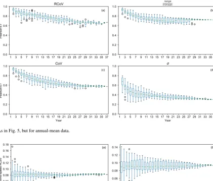
the wind farms. Therefore, the compact collection of wind-speed and energy-production IAVs causes strong correla-tions, solely because of the small number of annual averages used in the IAV calculation. Thus, the correlations via annual means demonstrate a downward trend with increasing length of data, regardless of the variability metrics chosen (Fig. 7). Although the correlations approach the 37-year values, the weakening correlations with more years included in the IAV calculations imply that using less data is preferred in con-necting the two IAVs. Note that the spread cannot be com-puted with one data point and hence the correlations between wind-speed IAVs and energy IAVs do not exist with a single year of data (Fig. 7). Overall, the asymptote analysis causes deceptive results, and, given the nature of the annual data, we cannot determine the sufficient length of data to effec-tively link the IAVs of wind speed and energy production. In other words, relating wind-speed IAV and energy-generation IAV with annual-mean data is flawed.
3.3 Wind-speed RCoV calculation and spatial distribution
Now that we have established that RCoV is a powerful and accurate way to relate wind-speed and energy-generation variations, we assess the required amount of data to
calcu-late the RCoV of wind speed. We compute the site-specific RCoVs using different spans of monthly mean wind speeds, including the OR and the TX sites (Fig. 8). The variations of RCoVs decrease as more years are included in the calcu-lations, and for each location we use the 37-year wind-speed RCoV as the long-term benchmark. For example, the 37-year wind-speed RCoV of 0.082 at the OR site means that the me-dian among the absolute deviations from the meme-dian is 8.2 % of the median monthly mean wind speed (Fig. 8a and Ta-ble 2). We determine the 37-yearσ’s as 10 % and 5 % of the 37-year RCoV, and we apply theχ2 approach at 90 % and 95 % confidence levels, respectively, to derive the conver-gence years, or the minimum length of wind-speed data re-quired to calculate RCoV effectively. The convergence years of the OR and TX sites are 12 and 25 years with a 90 % con-fidence, and 20 and 31 years with a 95 % concon-fidence, respec-tively (Table B5). In other words, for the OR site, one needs 12 years of monthly mean wind speeds to compute RCoV with a 90 % confidence that the resultant RCoV is within a 10 % deviation from the 37-year RCoV.
1 3 5 7 9 11 13 15 17 19 21 23 25 27 29 31 33 35 37 0.0
0.2 0.4 0.6 0.8 1.0
Pearson's r
(a) RCoV
1 3 5 7 9 11 13 15 17 19 21 23 25 27 29 31 33 35 37
0.0 0.2 0.4 0.6 0.8 1.0
(b) range
t rim ean
1 3 5 7 9 11 13 15 17 19 21 23 25 27 29 31 33 35 37
Year 0.0
0.2 0.4 0.6 0.8 1.0
Pearson's r
(c) CoV
1 3 5 7 9 11 13 15 17 19 21 23 25 27 29 31 33 35 37
Year 0.0
0.2 0.4 0.6 0.8 1.0
(d)
Figure 7.As in Fig. 5, but for annual-mean data.
1 3 5 7 9 11 13 15 17 19 21 23 25 27 29 31 33 35 37 Years of analysis period
0.04 0.06 0.08 0.10 0.12 0.14 0.16 0.18
Wind-speed RCoV
1 3 5 7 9 11 13 15 17 19 21 23 25 27 29 31 33 35 37 Years of analysis period
0.04 0.06 0.08 0.10 0.12 0.14
(a) (b)
Figure 8.Box plots of wind-speed RCoV using monthly MERRA-2 data for different time frames from 1 year to 37 years at(a)the OR site and(b)the TX site.
included in the RCoV calculation (Fig. 9a). For each grid point, the sample size of RCoV also becomes smaller, from 37 RCoVs of 1 year of data to 1 RCoV of 37 years of data, and hence theσ of RCoV decreases as the length of the anal-ysis period of wind speed increases (Fig. 9a). With theσ’s of RCoVs across 37 years, we determine the convergence years via theχ2method. For a certain confidence level, the cumu-lative fraction of the CONUS grid cells that exceed the asso-ciated threshold ofχ2-derived confidence intervals increases with the length of data (Fig. 9b). Among all of the MERRA-2 grid cells in the CONUS, the median convergence year is 10 years and the associated MAD is 3 years at a 90 % con-fidence level (Fig. 9b and Table B5). In other words, to as-sess the wind-speed variability via RCoV with a maximum of 10 % error from the long-term value and a 90 % confidence, one needs 10±3 years of monthly mean wind-speed records.
1 3 5 7 9 11 13 15 17 19 21 23 25 27 29 31 33 35 37 Year
0.00 0.01 0.02 0.03 0.04 0.05 0.06
o
f
R
C
o
V
(a)
5 10 15 20 25 30 35
Year 0
20 40 60 80 100
U.S. grid cells satisfying threshold (%)
(b) Monthly; 90 % confidence
Monthly; 95 % confidence Annual; 90 % confidence Annual; 95 % confidence
Figure 9.(a)Box plots ofσ’s of wind-speed RCoVs, where the RCoVs are calculated using monthly mean MERRA-2 data of 1 to 37 years. For each year, each box summarizes theσ from each MERRA-2 grid cell in the CONUS;(b)the time series of the cumulative fraction of grid cells in the CONUS that satisfies the threshold: when the pair of theχ2-derivedσ’s from the grid cell, calculated using the particular amount of data, become smaller than the 37-yearσ. The solid black, dash black, solid orange, and dash orange lines, respectively, indicate the minimum length of data: when the wind-speed RCoV using monthly mean data yields a 10 % deviation at maximum from the 37-year value at a 90 % confidence level, when the wind-speed RCoV using monthly mean data yields a 5 % deviation at maximum from the 37-year value at a 95 % confidence level, when the wind-speed RCoV using yearly mean data yields a 10 % deviation at maximum from the 37-year value at a 90 % confidence level, and when the wind-speed RCoV using yearly mean data yields a 5 % deviation at maximum from the 37-year value at a 95 % confidence level.
Spatial distributions of wind-speed RCoVs across the CONUS identify locations with reliable wind resources. Based on the site-specific convergence years at a 90 % confi-dence level (Fig. 10a), we calculate the RCoVs with monthly mean wind speeds of the particular time spans at each grid point and normalize with the CONUS median (Fig. 10b). Re-gions requiring long wind-speed records are irregularly scat-tered across the continent, such as the Northeast, the Dakotas, and Texas. The mountainous states generally illustrate high RCoVs, including the Appalachians and the Rockies. Given the strong correlations between the wind-speed RCoV and energy-production RCoV, Fig. 10b offers a realistic estima-tion of the general spatial pattern of the variability in wind-energy production as well. Note that, qualitatively, Fig. 10b is similar to the maps of wind-speed variability in Fig. 13a of Gunturu and Schlosser (2012) and in Fig. 3 in Hamling-ton et al. (2015), which also illustrate the variability of wind resources in the CONUS. In addition, using a 10-year fixed
length of wind-speed data for all CONUS grid points to com-pute RCoV results in a nearly identical spatial distribution to the pattern in Fig. 10b.
Further, an ideal location for wind farms should exhibit ample wind speeds with low variability. We combine the spa-tial variations of the normalized RCoV and the long-term wind resource (Fig. 10b and c), and we differentiate regions according to the CONUS median RCoV and wind speed (Fig. 10d). Favorable candidates for wind farm developments have above-average wind speeds and below-average variabil-ities, such as the Plains, parts of the upper Midwest, spots in the Columbia River region, and pockets nears the coasts of the Carolinas; poor places for wind power with weak winds and strong variabilities include the Appalachians and most of the Northeast.
Figure 10.(a)Map of the convergence years, or years of monthly mean wind-speed data required to derive a maximum of 10 % deviation from the 37-year RCoV at each grid point, at a 90 % confidence level. The CONUS median is 10 years with the MAD of 3 years;(b)map of RCoV of monthly mean wind speed using the grid-cell-specific convergence years in(a), normalized using the CONUS RCoV median at 0.100. The RCoVs illustrated are averaged over (37−convergence year+1) available year blocks. The MAD of the normalized RCoV in the CONUS is 0.224;(c)map of the mean monthly wind speed at 80 m of 37 years from 1980 to 2016. The CONUS median is 6.45 m s−1with the MAD of 1.03 m s−1;(d)map of wind resource and its variability, by summarizing(b)and(c)into four categories: regions with below-median wind speed and above-below-median RCoV (grey), regions with below-below-median wind speed and below-below-median RCoV (orange), regions with above-median wind speed and above-median RCoV (orange red), and regions with above-median wind speed and below-median RCoV (dark red), based on the CONUS median wind speed and RCoV.
do not demonstrate any geographical pattern as in Fig. 10a. Additionally, when using RCoV to represent IAV, the spatial patterns of required data lengths and the resultant normal-ized RCoVs for annual data are notably different from the monthly mean results, and geographical features seem to be irrelevant (Fig. A3). Furthermore, the categorical features of CoV resemble those of RCoV for onshore wind resources in the CONUS, whereas usingσresults in notably distinct clas-sifications of CONUS wind resources (Figs. 10d and A4).
4 Discussion
When using statistically robust and resistant variability met-rics, higher correlations between variabilities of wind speed and energy production emerge. Statistically robust methods do not assume or require any underlying wind-speed distri-butions, and statistically resistant methods are insensitive to wind-speed extremes. Of all methods, three robust and
re-sistant metrics, RCoV, MAD divided by trimean, and IQR divided by median, result in the largest threer’s in Tables 3 and B1, which suggests that they are the most useful met-rics to quantify long-term variability. Depending on the me-teorological data availability, wind-speed characteristics, and terrain complexity, different methods are appropriate in dif-ferent conditions. Nevertheless, robust and resistant meth-ods are best able to relate wind-speed variability and energy-generation variability, and RCoV is the most effective of all the metrics.
peri-ods of 2 to 6 years to yield strong wind-speed and energy-production correlations (Table 3). Even though different lo-cations require various spans of data (Fig. 10a), the average of the resultant RCoVs using 10 years of wind speeds leads to nearly identical spatial distributions (Fig. 10b). Therefore, to effectively quantify wind-speed variability and thus ade-quately derive energy-generation variability, we recommend using the RCoV with 10 years of monthly mean wind-speed data.
Annual-mean data are inadequate to relate wind-speed and energy-production IAVs or to represent wind-speed IAVs. We cannot determine the minimum years of data to relate an-nual wind-speed and energy IAVs because their correlations decline with the length of data (Fig. 7). Moreover, the coarse time resolution of annual averages smooths out the fluctua-tions of smaller timescales. Yearly mean wind speeds also possess different distribution characteristics, such as skew-ness and kurtosis, compared to those of finer temporal res-olutions (Lee et al., 2018). The nonzero kurtosis and skew-ness in Table 2 and in Lee et al. (2018) illustrate that most of the distributions of annual-mean wind speeds in the CONUS are non-Gaussian. Hence, using nonrobust metrics, such as σ, to evaluate IAV with samples of annual means from non-Gaussian distributions can lead to incorrect representations of variability.
Additionally, extended years of wind-speed data are also necessary to compute RCoV and represent IAV (Fig. A3a), and the resultant IAVs (Fig. A3b) differ from the variabili-ties calculated via monthly wind speeds (Fig. 10b). For in-stance, the low IAVs in the Appalachians (Fig. A3b) calcu-lated with yearly mean wind speeds contradict the pattern of high monthly mean wind-speed RCoVs in mountainous areas (Fig. 10b) as well as the findings in past research (Gun-turu and Schlosser, 2012; Hamlington et al., 2015). Further-more, some of the grid points require more than 37 years of yearly mean data to calculate wind-speed RCoV with statis-tical confidence (Fig. 9 and Table B5). Although RCoV does not yield the strongest 37-yearr in relating wind-speed and energy IAVs, readers should be cautious when using a lim-ited number of annual-mean data to derive IAVs. In short, to effectively assess the long-term variability of wind farm pro-ductivity, one should use wind speeds finer than yearly mean data.
Regions with ample wind resources and low variability favor wind-energy developments, coinciding with the loca-tions of many existing wind farms in the CONUS (Fig. 10d). Wind farms in the Plains and parts of the upper Midwest benefit from the above-average wind speeds and the below-average wind-speed RCoVs. Other regions, such as parts of the Columbia River region and the Carolinas, also experience strong, consistent winds. The Northeast and the Appalachi-ans are relatively unfavorable for producing a stable, onshore wind-energy supply, whereas the area east of Cape Cod in Massachusetts and the sections along the West Coast exhibit a promising offshore wind resource. Wind farm developers
should account for wind resource as well as its long-term variability in repowering existing turbines and building new wind farms.
Furthermore, mathematically, a normalized spread metric, namely a spread statistic divided by an average metric, is more useful than solely a spread metric in assessing variabil-ity, and a normalized spread metric should always be pre-sented with the corresponding averaging metric. For exam-ple, RCoV and CoV between wind speed and energy yield largerr’s than MAD and σ (Table 3 and Fig. A1), and the r’s between wind-speed RCoV and CoV are also higher than those comparisons involving MAD andσ(Fig. 6). Forσ, the root mean square of the deviation from the mean is not sta-tistically robust or resistant, and 1σ means the uncertainty is 18.3 % from the mean. Hence, CoV, or theσ divided by the mean, is the respective normalized uncertainty metric toσ. For instance, the wind-speed CoVs of both the OR and TX sites are about 0.13 (Table 2), implying theσ is 13 % from the mean. In contrast, using RCoV, or the MAD divided by the median, is a robust and outlier-resistant metric of normal-ized uncertainty. For example, the wind-speed RCoVs of the OR and TX sites are 0.08 and 0.09, respectively (Table 2), in-dicating the MADs are 8 % and 9 % from their median wind speeds. Even though RCoV is not as commonly used and not as intuitive asσ or CoV, RCoV is unrestricted by any un-derlying distribution assumptions. Overall, to correctly and effectively use the normalized spread metrics, both the nor-malized spread metric and the average value need to be stated clearly in pairs. In other words, the interpretation of “the variability is 2 %” oversimplifies the statistics of uncertainty quantification. Therefore, we recommend presenting both the RCoV and the median of a time series together in estimating variability.
5 Conclusions
Wind-speed variability is a crucial component in assessing the overall uncertainty of P50, which is the estimated aver-age energy production of a wind farm. This study highlights the importance of using rigorous methods to estimate inter-monthly and interannual variability. To search for suitable ways to quantify this uncertainty under different conditions, we investigate 27 combinations of spread metrics over 607 wind farms in the United States, with closer examination of two geographically distinct sites. We evaluate the meth-ods for robustness to non-Gaussian distributions and resis-tance to extreme values, in contrast to the common practice of using only standard deviation (σ). We calculate variabil-ities using monthly and annual mean wind speeds from the MERRA-2 reanalysis data set and wind farm monthly net en-ergy production from the EIA. We find that within the con-tiguous United States (CONUS), statistically robust and re-sistant methods predict variabilities more accurately, partic-ularly in that wind-speed variabilities strongly correlate with observed energy-production variabilities.
We recommend using the robust coefficient of variation (RCoV) to quantify variabilities of wind resource and en-ergy production. RCoV, defined as the median of absolute deviation from the median wind speed divided by the me-dian of the wind speed, is a robust and resistant spread met-ric, in contrast toσ. RCoV yields strong correlations consis-tently (a Pearson’s correlation coefficient, or a Pearson’sr, of 0.856 with 37 years of monthly means) in various sensi-tivity tests via different correlation coefficients, whereas σ does not. In other words, using RCoV, a wind farm with high wind-speed fluctuations also possesses high variations in wind-energy generations and vice versa, whereas other metrics do not reflect that relationship as effectively. RCoV, as a normalized spread metric, also leads to a more accurate depiction of wind-speed variabilities thanσ, a simple spread metric. Contrary to the custom of displaying uncertainty in one percentage value, we advise users to assess both the RCoV and the median in estimating intermonthly variability. Moreover, depending on the location, on average 10±3 years of monthly speed data are necessary to compute wind-speed RCoV with a 90 % statistical confidence, such that the resultant RCoV deviates within 10 % of the long-term RCoV.
RCoV characterizes the spreads of the distributions of wind resources and wind-energy production. The relatively low monthly mean wind-speed RCoVs in the central United States indicate stable long-term wind resources, and the RCoV overall spatial distribution in the CONUS agrees with the findings from past research. Other distribution diagnos-tics, such as kurtosis and skewness, also result in strong correlations between monthly mean wind speed and en-ergy generation, and thus they adequately represent enen-ergy- energy-production characteristics.
Because the long-term correlations between the wind-speed and energy-production interannual variabilities (IAVs) are weak (a Pearson’srof 0.668 for RCoV with 37 years of data) and decrease with the length of data, we cannot deter-mine the minimum length of annual mean data required for skillful assessment of IAV. Hence, we do not recommend cal-culating IAVs with annual-mean data. Although the concept of IAV has been essential in determining the annual energy production in the wind resource assessment process, annual-mean wind speeds mask signals of finer temporal scales and thus lead to unreliable representations of long-term variabil-ity. Overall, uncertainty arises in the process of calculat-ing IAVs based on limited samples, whereas RCoV yields credible intermonthly variabilities considering the adequate amount of monthly mean data.
Now that we have highlighted the preferred structure of using RCoV, we can assess finer-scale variations us-ing high-resolution wind-speed and energy-production data. With data of different temporal scales, the autocorrelation of wind resources and its relationship with long-term energy-production variations can also be quantified. The influence of climatic cycles on energy production can be explored. Fur-thermore, applying the concept of RCoV to reduce the uncer-tainty of P50 and assist financial decisions can be beneficial to the industry.
Appendix A
0.01 0.02 0.03
Yearly mean wind-speed RCoV 0.01 0.02 0.03 0.04 0.05 0.06
Yearly mean energy-production RCoV
(a)
r = 0.668
0.10 0.15 0.20 0.25
Yearly m ean wind-speed t rim eanrange
0.1 0.2 0.3 0.4 Y e a rl y m e a n e n e rg y -p ro d u ct io n ra n g e tr im e a n (b)
r = 0.719
0.01 0.02 0.03 0.04 0.05
Yearly mean wind-speed CoV 0.02
0.04 0.06 0.08 0.10
Yearly mean energy-production CoV
(c)
r = 0.573
0.10 0.15 0.20 0.25 0.30 0.35
Yearly m ean wind-speed 0 1 2 3 4 5 Y e a rl y m e a n e n e rg y -p ro d u ct io n (d)
r = 0.305
Figure A1.As in Fig. 4, but the metrics are calculated using annual-mean wind speed and energy production.
0.01 0.02 0.03 0.04 0.05 Yearly mean wind-speed CoV 0.00
0.01 0.02 0.03
Yearly mean wind-speed RCoV
(a)
r = 0.497
rs = 0.514
= 0.35
0.05 0.10 0.15 0.20 Yearly mean wind-speed MAD 0.00
0.01 0.02 0.03
Yearly mean wind-speed RCoV
(b)
r = 0.895
rs = 0.867
= 0.723
0.01 0.02 0.03 0.04 0.05 Yearly mean wind-speed CoV 0.10 0.15 0.20 0.25 0.30 0.35 Y e a rl y m e a n w in d -s p e e d (c)
r = 0.871
rs = 0.895
= 0.747
0.05 0.10 0.15 0.20 Yearly mean wind-speed MAD 0.10 0.15 0.20 0.25 0.30 0.35 Y e a rl y m e a n w in d -s p e e d (d)
r = 0.653
rs = 0.725
= 0.531
Figure A3.As in Fig. 10a and b, but the data plotted are annual-mean wind speeds:(a)map of the convergence years, or years of wind-speed data required to derive a maximum of 10 % deviation from the 37-year RCoV at each grid point at a 90 % confidence level. Because 12.6 % of the CONUS grid points yield convergence years beyond 37 years using annual data (solid orange line in Fig. 9 and first column in Table B5), we assign 37 years as the convergence years for those grid points. After excluding the non-numeric values, the CONUS median is 27 years and the MAD is 4 years;(b)map of RCoV of annual-mean wind speed using the grid-cell-specific convergence years in(a), normalized using the CONUS RCoV median at 0.020. The RCoVs illustrated are averaged over (37−convergence year+1) available year blocks. The MAD of the normalized RCoV in the CONUS is 0.205.
(a)
Below-median wind speed, above-median variability
Below-median wind speed, below-median variability
Above-median wind speed, above-median variability Above-median wind speed, below-median variability
(b)
CoV
Appendix B
Table B1.Description of the 26 spread metrics tested, adapted from Wilks (2011), and the 37-yearr’s from ther-filtered monthly data. q0.25is the 25th percentile (first quartile),q0.5is the 50th percentile (median), andq0.75is the 75th percentile (third quartile). Trimean=
1
4(q0.25+2×q0.5+q0.75), range(x)=max (x)−min(x), and an overbar (x) indicates the arithmetic mean. Reason I: the metric is not robust
because the metric possesses distribution constraints, for example, assuming a Gaussian distribution, and the metric is not resistant because outliers influence it; Reason II: the metric is not resistant because outliers influence it; Reason III: the numerator of the metric is not robust or resistant; Reason IV: the denominator of the metric is not robust or resistant; Reason V: the numerator of the metric is not resistant.
Spread metrics 37-year Robust and Why not robust
r resistant and resistant
Interquartile range (IQR)=q0.75−q0.25 0.214 Yes –
IQR
median 0.845 Yes –
IQR
trimean 0.834 Yes –
Median deviation from median=median[x−median (x)] −0.048 Yes –
Median absolute deviation (MAD)=median|x−median (x)| 0.196 Yes –
Robust coefficient of variation (RCoV)= MAD
median 0.856 Yes –
Exponential RCoV= ln(MAD)
ln(median) 0.595 Yes –
MAD
trimean 0.848 Yes –
Standard deviation (σ)=
s 1 n−1
n P
i=1
(xi−x)2 0.184 No Reason I
Variance (σ2)= 1
n−1 n P
i=1
(xi−x)2 0.136 No Reason I
Coefficient of variation (CoV)= σ
mean 0.704 No Reason I
Exponential CoV= ln(σ)
ln(mean) 0.466 No Reason I
Mean deviation from mean=(x−x) −0.043 No Reason I
Mean absolute deviation= |x−x| 0.187 No Reason I
Trimmed standard deviation (σ)=standard deviation without values belowQ10and Q90,or =
s 1 n−2k
n−k P
i=k+1
x(i)−xa2, kas the nearest integer toa×n
0.206 No Reason I
Trimmedσ
x 0.775 No Reason I
Range 0.177 No Reason II
Range
x 0.609 No Reason I
Seasonality index=
P|
x−x|
n×x (modified from Walsh and Lawler, 1981) 0.744 No Reason I
σ
median 0.743 Partially Reason III
σ
trimean 0.728 Partially Reason III
IQR
x 0.818 Partially Reason IV
MAD
x 0.834 Partially Reason IV
Trimmedσ
median 0.806 Partially Reason III
Trimmedσ
trimean 0.794 Partially Reason III
Range
median 0.650 Partially Reason V
Range
Table B2.Description of the distribution diagnostics tested, adapted from Wilks (2011) and the 37-yearr’s from ther-filtered monthly data. Reason I: the metric is not robust because the metric possesses distribution constraints, for example, assuming a Gaussian distribution, and the metric is not resistant because outliers influence it; Reason II: the metric is not robust because it assumes a Weibull distribution.
Other diagnostics Description 37-year Robust and Why not robust r resistant and resistant
Kurtosis (tailedness)=
1 n
n P
i=1
(xi−x)4
(n1 n P
i=1
(xi−x)2)2
−3
Positive value means the distribution is tail heavy with more and more ex-treme outliers compared to Gaussian; vice versa
0.936 No Reason I
Skewness= 1 n n P
i=1
(xi−x)3
(1n
n P
i=1
(xi−x)2) 3 2
Positive value means long right tails, or right skewed; vice versa
0.943 No Reason I
Yule–Kendall Index (YKI)= q0.25−2×q0.5+q0.75
IQR
Positive value means long right tails, or right skewed; vice versa
0.778 Yes –
Weibull scale parameter Determine the peak and the stretch 0.379 No Reason II Weibull shape parameter Determine the average, the symmetry,
and the shape
0.721 No Reason II
Autocorrelation Pearson’srwith its own past and future values
Not applicable Not applicable –
Table B3.As in Table 3, but with the calculated metrics, the associated correlations, and asymptote periods using differentR2andrfilters and adding the randomized standard error to predicted monthly total energy production. The sample sizes of the 0.7-r threshold test, the 0.9-rthreshold test, and the random error test are 306, 83, and 195 wind farms, respectively.
Sensitivity test R2=0.6 R2=0.85 Random error r=0.7 r=0.9
Spread metrics 37-yearr Asymptote years 37-yearr Asymptote years 37-yearr Asymptote years
CoV 0.650 6 0.787 3 0.675 6
σ
median 0.682 5 0.820 2 0.708 4
σ
trimean 0.671 5 0.804 3 0.695 5 IQR
mean 0.786 4 0.837 3 0.774 7
IQR
median 0.811 3 0.865 2 0.799 6 IQR
trimean 0.801 4 0.851 3 0.789 7
RCoV 0.815 3 0.879 2 0.808 6
MAD
mean 0.793 3 0.859 3 0.786 7
MAD
trimean 0.807 3 0.870 3 0.800 6 Range
mean 0.524 31 0.767 26 0.567 29
Trimmedσ
median 0.736 5 0.816 3 0.741 6 Trimmedσ
trimean 0.753 4 0.831 3 0.758 5 Seasonality index, modified from
Walsh and Lawler (1981)
0.695 5 0.804 3 0.710 5
Other diagnostics
Kurtosis 0.896 5 0.927 1 0.886 14
Skewness 0.931 1 0.951 1 0.918 8
YKI 0.756 23 0.833 19 0.669 25
Table B4.As in Table 3, but with the calculated metrics, the associated correlations, and asymptote periods using annual-mean wind speed and energy production using the 195r-filtered sites.
Spread metrics 37-yearr Asymptote years
CoV 0.573 27
σ
median 0.567 27
σ
trimean 0.569 27
IQR
mean 0.699 24
IQR
median 0.697 24
IQR
trimean 0.699 24
RCoV 0.668 27
MAD
mean 0.670 25
MAD
trimean 0.670 25
Range
mean 0.723 27
Trimmedσ
median 0.567 27
Trimmedσ
trimean 0.569 27
Seasonality index, modified from Walsh and Lawler (1981) 0.547 29
Other diagnostics
Kurtosis 0.985 5
Skewness 0.980 4
YKI 0.853 12
Weibull shape parameter 0.649 28
Table B5.Convergence years based on theχ2approach of wind-speed RCoV (as in Figs. 8 and 9), wind-speed CoV, and wind-speedσ, using monthly and yearly wind speeds. The calculations of median and MAD exclude the data with convergence years beyond 37 years in the CONUS.
Monthly mean wind speed RCoV CoV σ
Confidence level 90 % 95 % 90 % 95 % 90 % 95 %
37-year sample size (of 5049 grid points) 5049 4923 5049 5039 5049 5048
Convergence years – CONUS median 10 20 4 12 4 12
Convergence years – CONUS MAD 3 4 2 5 2 5
Convergence years – OR site 12 20 6 15 6 15
Convergence years – TX site 25 31 7 24 5 24
Yearly mean wind speed RCoV CoV σ
Confidence level 90 % 95 % 90 % 95 % 90 % 95 %
37-year sample size (of 5049 grid points) 4414 2565 5034 4292 5034 4301
Convergence years – CONUS median 27 33 20 28 19 28